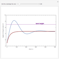
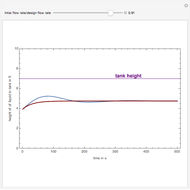
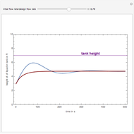
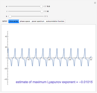
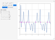
Dynamic Simulation of a Gravity-Flow Tank
Initializing live version


Requires a Wolfram Notebook System
Interact on desktop, mobile and cloud with the free Wolfram Player or other Wolfram Language products.
The dynamic behavior of a tank and pipe system is described by the following coupled ordinary differential equations:
[more]


Contributed by: Housam Binous (March 2011)
Open content licensed under CC BY-NC-SA
Snapshots


Details
W. L. Luyben, Process Modeling, Simulation and Control for Chemical Engineers, 2nd ed., New York: McGraw-Hill International Editions, 1996.
Permanent Citation
Related Demonstrations
More by Author
 Dynamic Behavior of a Heated Stirred Tank
Housam Binous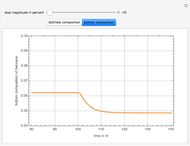 Dynamic Simulation of a Binary Distillation Column
Housam Binous Dynamic Behavior of Heated Tanks in Series
Housam Binous and Ahmed Bellagi Dynamic Behavior of Three Tanks in Series
Housam Binous, Brian G. Higgins, and Ahmed Bellagi Dynamic Behavior of a Bioreactor
Housam Binous Action of a Continuous Stirred-Tank Reactor
Housam Binous and Ahmed Bellagi Dynamic Behavior of Isothermal Flash Vessel
Housam Binous and Ahmed Bellagi Dynamic Behavior of a Nonisothermal Chemical System
Housam Binous and Zakia Nasri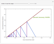 Cross-Flow Liquid-Liquid Extraction
Housam Binous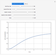 Two Isothermal Continuous Stirred-Tank Reactors with a Recycle Stream
Housam Binous and Ahmed Bellagi
-
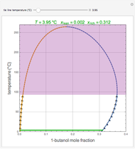 Liquid-Liquid Equilibrium for the 1-Butanol-Water System
Housam Binous -
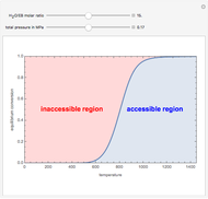 Temperature Dependence of Dehydrogenation of Ethyl Benzene to Styrene
Housam Binous -
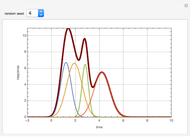 Deconvolution of a Chromatogram
Housam Binous -
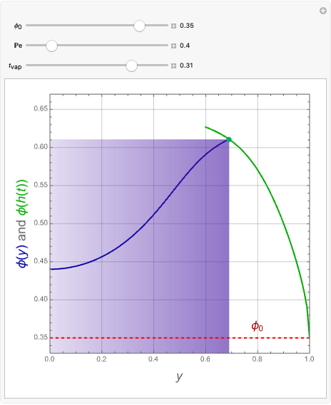 Distribution of Colloidal Particles during Solvent Evaporation
Housam Binous -
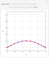 Heat Conduction in a Rod
Housam Binous -
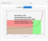 Optimal Setup of Two Continuous Stirred-Tank Reactors (CSTRs) in Series
Housam Binous -
 Study of the Dynamic Behavior of the Lorenz System
Housam Binous -
 A Graphically Enhanced Method for Computing Real Roots of Nonlinear Functions
Housam Binous -
 Design of a Shell and Tube Heat Exchanger
Housam Binous -
 Correction Factor for Shell and Tube Heat Exchanger
Housam Binous -
 Contour Plots for Reaction Rates
Housam Binous -
 Optimal Conditions for CO2/n-Hexane Flash Separation
Housam Binous -
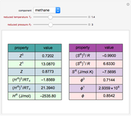
 Residual Functions for the SRK and PR Equations of State
Housam Binous -
 Gas-Phase Fugacity Coefficients for Propylene
Housam Binous -
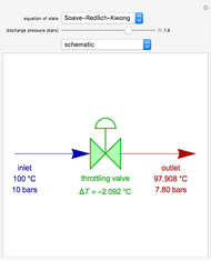 Operation of a Throttling Valve
Housam Binous -
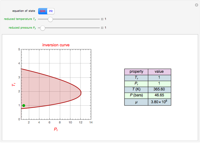 Joule-Thomson Inversion Curves for Soave-Redlich-Kwong (SRK) and Peng-Robinson (PR) Equations of State
Housam Binous -
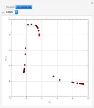
 Lee-Kesler Generalized Correlations for Gases
Housam Binous -
 Mapping the Maxima for a Nonisothermal Chemical System
Housam Binous -
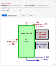 Operation of an Air Conditioner
Housam Binous -
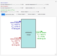 Adiabatic Mixing of Two Moist Air Streams
Housam Binous