Uncertainty in Sonar Performance Prediction


Requires a Wolfram Notebook System
Interact on desktop, mobile and cloud with the free Wolfram Player or other Wolfram Language products.
Sonar performance prediction can be viewed as a two-step process. In the first step, the statistical properties of the signal and noise fields at the sonar are estimated. The characteristic parameter is the signal to noise ratio ( ). In the second stage,
  is converted to probability of detection
  using a mapping appropriate to the sonar type and method of operation. If the
  is known exactly then, the probability of detection
  is a number on the interval
  . As a practical matter
  is never known with total certainty. This Demonstration illustrates the effect of uncertainty in
  on the estimation of probability of detection
  .
.
Contributed by: Marshall Bradley (March 2011)
Open content licensed under CC BY-NC-SA
Snapshots


Details
In underwater acoustics, sonar performance is predicted with the aid of the sonar equation. A simple example of a sonar equation expressed on a decibel scale applicable to passive sonar is the following:  , where
  is the signal to noise ratio (dB),
  is the target source level (dB re 1 μPa at 1m),
  is the transmission loss (dB re 1 m), and
  is the ambient noise level (dB re 1
  ). In practical situations the individual terms in the sonar equation are not precisely known. Thus there is uncertainty associated with an
  prediction.
If we let  denote the
  , then a plausible initial assumption is that
  is a normally distributed random variable with probability density function
 ,
,
where  is the mean decibel
  level predicted by the modeling process and
  is the measure of the decibel uncertainty associated with the prediction. For example, in a situation where acoustic performance prediction models predict favorable sonar performance with high certainty, we might have
  and
and  . If we let the random variable
  denote the signal to noise ratio measured on an intensity scale, then the relationship between the random variables
  and
and  is
is

 InlineMath, InlineMath
The random variable  is said to have a lognormal distribution and its probability density function is
 .
.
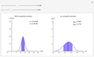
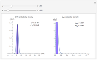
The probability density functions  and
and  convey the same information about the uncertainty in
  , only the scales are different. When measured on an intensity scale,
  is defined on the interval
  . If we measure
  on a decibel scale, then it is defined on the interval
  . The condition of absolutely no signal corresponds to
  or
or  .
.  Infinite signal corresponds to infinity on both scales.
If we assume that the sonar is optimized for a signal with random phase and Rayleigh amplitude, then the appropriate mapping from  to probability of detection
  is ([1])
 ,
,
where  is the sonar false alarm rate and
  is the
  measured on an intensity scale. The function
  is a monotonic increasing map from intensity
  to probability of detection. It has the inverse function
 ,
,
with derivative
 .
.
Because of the simple properties of the inverse function  , the probability density function
  of probability of detection
  can be found in closed form. The result is
 ,
,
or more completely
 ,
,  .
.
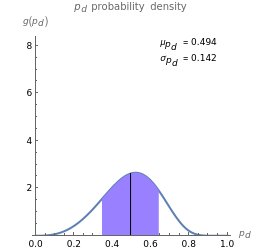
Due to the uncertainty in  , the probability of detection
  is no longer a single number but rather a statistical distribution. The expected value and variance of the probability of detection are useful characterizations of this distribution. They are defined to be
 ,
,
 .
.
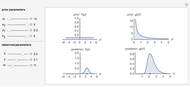
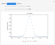
Use the two sliders to control the selection of  the mean
  (dB) and
  the standard deviation of
  (dB). When
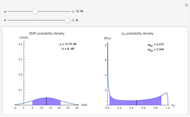
  is small, the distribution of probability of detection is peaked with a relatively small standard deviation (square root of variance). This is indicative of a useful prediction of probability of detection. However, when
  is larger, the distribution of probability of detection is much more spread out and has a much larger standard deviation. In this latter circumstance, the predicted probability of detection may not be useful due to the large associated uncertainty.
Reference
[1] A. D. Whalen, Detection of Signals in Noise, New York: Academic Press, 1971.
Permanent Citation
 High-Frequency Sonar Performance
Marshall Bradley Micro-Doppler Sonar Simulation
Marshall Bradley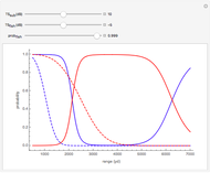 Bayesian Range Weighting for Sonar
Marshall Bradley Sonar
Sonar
Enrique Zeleny Frequency-Modulated Continuous-Wave (FMCW) Radar
Marshall Bradley Chladni Figures
Enrique Zeleny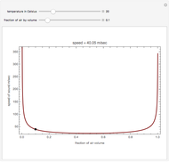 Speed of Sound in Water-Air Mixtures
Kay Herbert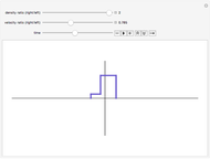 Reflection and Transmission of Acoustic Waves
David von Seggern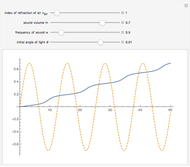 Path of Light through an Acoustic Wave
Brendon O'Leary Reverberations in Acoustic Layers
David von Seggern (University of Nevada)
-
 Bayesian Distribution of Sample Mean
Marshall Bradley -
 Fluid Flow around a Corner
Marshall Bradley -
 Underwater Vehicle Pressure Signature
Marshall Bradley -
 Extreme Value Forecasting
Marshall Bradley -
 Target Motion with the Metropolis-Hastings Algorithm
Marshall Bradley -
 Noise Temperature of a Radar System
Marshall Bradley -
High-Frequency Sonar Performance
Marshall Bradley -
 Atmospheric Radar Wave Absorption
Marshall Bradley -
 Equine Motion
Marshall Bradley -
Frequency-Modulated Continuous-Wave (FMCW) Radar
Marshall Bradley -
 Maximum Entropy Probability Density Functions
Marshall Bradley -
 Uncertainty in Sonar Performance Prediction
Marshall Bradley -
Micro-Doppler Sonar Simulation
Marshall Bradley -
 Human Walking Animation
Marshall Bradley -
Bayesian Range Weighting for Sonar
Marshall Bradley