Chebyshev Collocation Method for 2D Boundary Value Problems


Requires a Wolfram Notebook System
Interact on desktop, mobile and cloud with the free Wolfram Player or other Wolfram Language products.
Consider the 2D boundary value problem given by 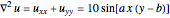 , with boundary conditions
  and
and  . You can set the values of
  and
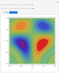
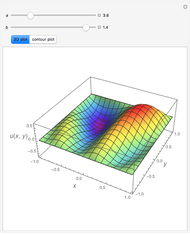
and  . Using this Demonstration, you can solve the PDE using the Chebyshev collocation method adapted for 2D problems. The solution is shown as either a 3D plot or a contour plot.
Contributed by: Housam Binous, Brian G. Higgins, and Ahmed Bellagi (March 2013)
Open content licensed under CC BY-NC-SA
Snapshots


Details
In the discrete Chebyshev–Gauss–Lobatto case, the interior points are given by  . These points are the extrema of the Chebyshev polynomial of the first kind,
  .
.
The  Chebyshev derivative matrix at the quadrature points is an
  matrix
  given by
 ,
,  ,
,  for
for 
and
 for
for  and
and  ,
,
where  for and
  .
.
The discrete Laplacian is given by  , where
  is the
  identity matrix,
  is the Kronecker product operator,
  , and
, and  is
is  without the first row and first column.
Reference
[1] L. N. Trefethen, Spectral Methods in MATLAB, Philadelphia: SIAM, 2000.
Permanent Citation
 Chebyshev Collocation Method for the Helmholtz Problem
Housam Binous, Brian G. Higgins, and Ahmed Bellagi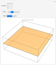 Convergence of Minimization Methods
Stephen Wolfram and Yifan Hu Minimizing the Rosenbrock Function
Michael Croucher Optimal Bin Packing with Random Lengths
Yifan Hu and Stephen Wolfram Chebyshev Collocation Method for Linear and Nonlinear Boundary Value Problems
Housam Binous, Brian G. Higgins, and Ahmed Bellagi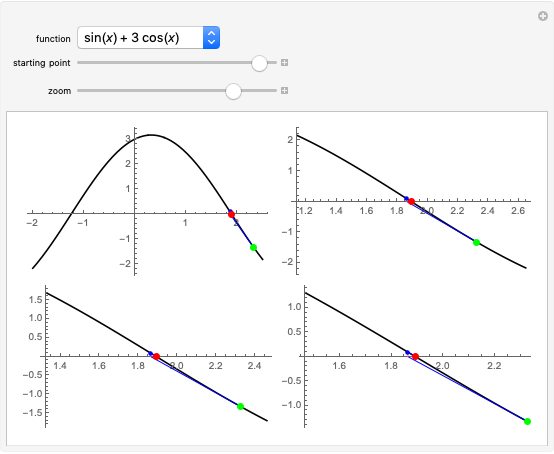 Newton's Method
Chris Maes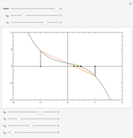 Secant Root Finding Method
Michael Trott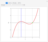 Peculiar Behavior of the Newton Method
Housam Binous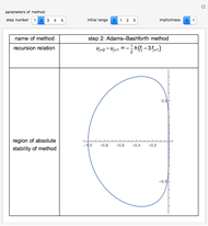 Linear Multistep Methods for First-Order ODEs
Wusu Ashiribo Senapon and Akanbi Moses Adebowale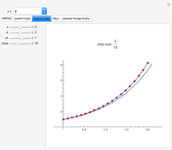 Numerical Methods for Differential Equations
Edda Eich-Soellner
-
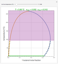 Liquid-Liquid Equilibrium for the 1-Butanol-Water System
Ahmed Bellagi -
 Temperature Dependence of Dehydrogenation of Ethyl Benzene to Styrene
Ahmed Bellagi -
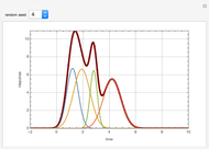 Deconvolution of a Chromatogram
Ahmed Bellagi -
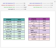 Design of a Shell and Tube Heat Exchanger
Ahmed Bellagi -
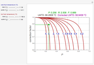 Correction Factor for Shell and Tube Heat Exchanger
Ahmed Bellagi -
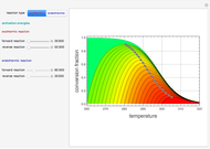 Contour Plots for Reaction Rates
Ahmed Bellagi -
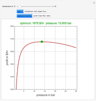 Optimal Conditions for CO2/n-Hexane Flash Separation
Ahmed Bellagi -
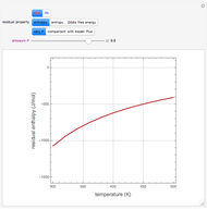 Residual Functions for the SRK and PR Equations of State
Ahmed Bellagi -
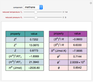
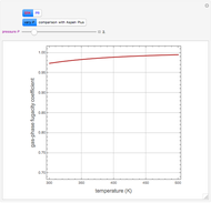 Gas-Phase Fugacity Coefficients for Propylene
Ahmed Bellagi -
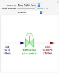 Operation of a Throttling Valve
Ahmed Bellagi -
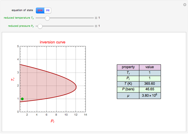 Joule-Thomson Inversion Curves for Soave-Redlich-Kwong (SRK) and Peng-Robinson (PR) Equations of State
Ahmed Bellagi -
 Lee-Kesler Generalized Correlations for Gases
Ahmed Bellagi -
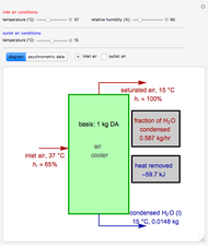 Operation of an Air Conditioner
Ahmed Bellagi -
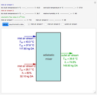 Adiabatic Mixing of Two Moist Air Streams
Ahmed Bellagi -
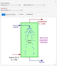 Adiabatic Humidification
Ahmed Bellagi -
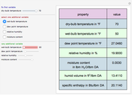 Psychrometric Data Calculator in English Engineering Units
Ahmed Bellagi -
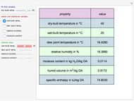 Psychrometric Data Calculator in SI Units
Ahmed Bellagi -
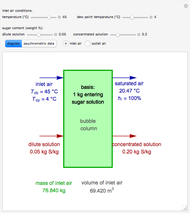 Concentration of Sugar Solution in a Bubble Column
Ahmed Bellagi -
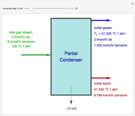 Operation of a Partial Condenser
Ahmed Bellagi -
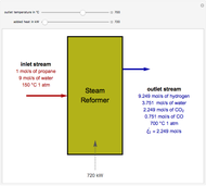 Steam Reforming of Propane
Ahmed Bellagi