Graphic Solution of a Second-Order Differential Equation


Requires a Wolfram Notebook System
Interact on desktop, mobile and cloud with the free Wolfram Player or other Wolfram Language products.
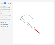
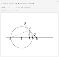
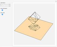
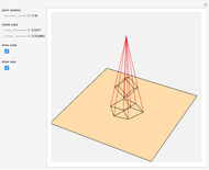
This Demonstration shows the Euler–Cauchy method for approximating the solution of an initial value problem with a second-order differential equation. An example of such an equation is  , with derivatives from now on always taken with respect to
  . This equation can be written as a pair of first-order equations,
  ,
,  .
.


Contributed by: Izidor Hafner (January 2014)
Open content licensed under CC BY-NC-SA
Snapshots


Details
References
[1] V. I. Smirnoff, Lectures in Higher Mathematics (in Russian), vol. 2, Moscow: Nauka, 1967 p. 50.
[2] L. Euler, "De Integratione Aequationum Differentialium Per Approximationem," Institutionum Calculi Integralis Volumen Primum, 1768. www.math.dartmouth.edu/~euler/docs/originals/E342sec2ch7.pdf.
Permanent Citation
 Smirnoff's Graphic Solution of a Second-Order Differential Equation
Izidor Hafner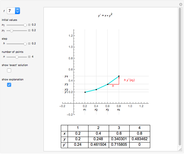 Graphic Solution of a First-Order Differential Equation
Izidor Hafner Numerical Solution of the Advection Partial Differential Equation: Finite Differences, Fixed Step Methods
Alejandro Luque Estepa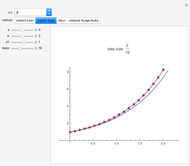 Numerical Methods for Differential Equations
Edda Eich-Soellner Solution of a PDE Using the Differential Transformation Method
Housam Binous, Ahmed Bellagi, and Brian G. Higgins Picard's Method for Ordinary Differential Equations
Oliver K. Ernst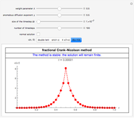 Numerical Solution of Some Fractional Diffusion Equations
Santos Bravo Yuste Solution of the Laplace Equation Using Coordinates Fitted to the Boundary Conditions
Brian G. Higgins and Housam Binous Mackey-Glass Equation
Rob Knapp Solution to Differential Equations Using Discrete Green's Function and Duhamel's Methods
Jason Beaulieu and Brian Vick
-
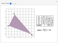 Area of a Polygon
Izidor Hafner -
 Pappus's Hexagons
Izidor Hafner -
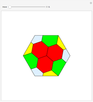 Freese's Dissection of a Regular Hexagon into Seven Hexagons
Izidor Hafner -
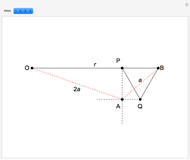 A Construction of the Square Root of Seven
Izidor Hafner -
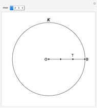
 The Apollonius Circle of a Triangle
Izidor Hafner -
 Freese's Dissection of a Regular Dodecagon into Six Squares
Izidor Hafner -
 Natural Language Neutral Symbolism in Propositional Logic
Izidor Hafner -
 Regressive Recursion
Izidor Hafner -
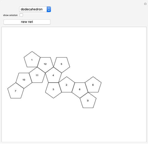
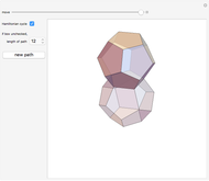
 Mazes on the Edges of a Polyhedron
Izidor Hafner -
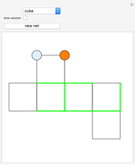
 Deduce the Net for a Die's Net
Izidor Hafner -
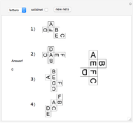
 Test Your Spatial Visualization Abilities
Izidor Hafner -
 Op Art on Golden Rhombic Solids (II)
Izidor Hafner -
 Golden Rhombic Solids with Nets
Izidor Hafner -
 Sum of the Squares of the Sides of a Projected Regular Tetrahedron
Izidor Hafner -
 Perspective Projection of a Cube onto a Plane
Izidor Hafner -
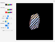
 Op Art on Platonic Solids
Izidor Hafner -
 Rolling a Regular Dodecahedron on a Congruent Dodecahedron
Izidor Hafner -
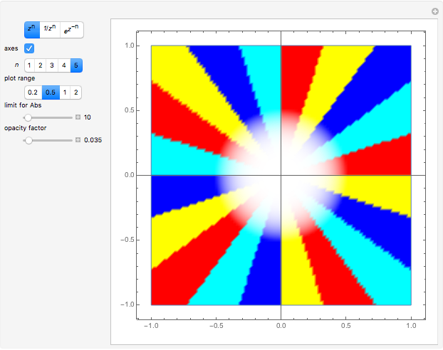 Zeros, Poles, and Essential Singularities
Izidor Hafner -
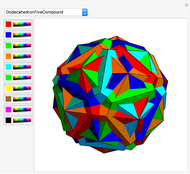 Polyhedral Compounds
Izidor Hafner -
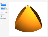 Meissner Tetrahedra
Izidor Hafner