A Domain Decomposition Method with Orthogonal Collocation


Requires a Wolfram Notebook System
Interact on desktop, mobile and cloud with the free Wolfram Player or other Wolfram Language products.
Consider the partial differential equation  with
with  and
and  , subject to the boundary and initial conditions
  ,
,  , and
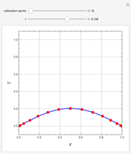
, and  . The solution
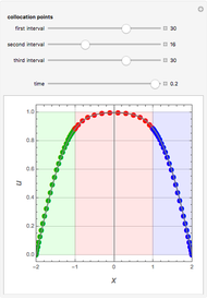
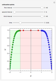
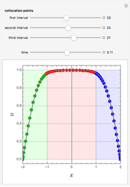
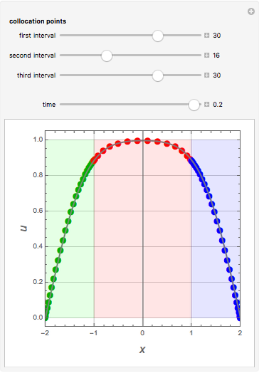
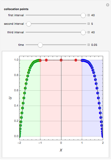
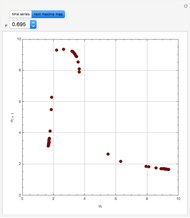
  is obtained using Mathematica's built-in function NDSolve (solid gray curve) and Chebyshev orthogonal collocation (colored dots). The interval
  is divided into three regions identified by the green, red, and blue panes. You can vary the number of Chebyshev collocation points in each region independently as well as the time,
  . The behavior of
  in the different panes dictates how many collocation points one has to choose from. Indeed, for small times the function
  is almost constant (equal to 1) in the red pane region and varies rapidly in the green and blue panes. This indicates that a small number of collocation points is required in the central region while a large number is required near the edges.
Contributed by: Housam Binous (July 2013)
Open content licensed under CC BY-NC-SA
Snapshots

Details
detailSectionParagraphPermanent Citation
"A Domain Decomposition Method with Orthogonal Collocation"
http://demonstrations.wolfram.com/ADomainDecompositionMethodWithOrthogonalCollocation/
Wolfram Demonstrations Project
Published: July 8 2013
 Chebyshev Collocation Method for Linear and Nonlinear Boundary Value Problems
Housam Binous, Brian G. Higgins, and Ahmed Bellagi Solution of a PDE Using the Differential Transformation Method
Housam Binous, Ahmed Bellagi, and Brian G. Higgins Eigenstates of the Quantum Harmonic Oscillator Using Spectral Methods
Housam Binous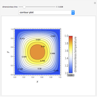 Transient Two-Dimensional Heat Conduction Using Chebyshev Collocation
Housam Binous, Brian G. Higgins, and Ahmed Bellagi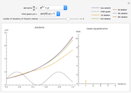 Picard's Method for Ordinary Differential Equations
Oliver K. Ernst Euler's Method for the Exponential Function
Arnaud Crouzet Numerical Methods for Differential Equations
Edda Eich-Soellner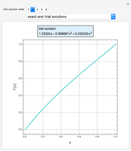 Boundary Value Problem Using Galerkin's Method
Housam Binous, Brian G. Higgins, and Ahmed Bellagi Absolute Stability of an Integration Method
Housam Binous, Brian G. Higgins, and Ahmed Bellagi Numerical Solution of the Advection Partial Differential Equation: Finite Differences, Fixed Step Methods
Alejandro Luque Estepa
-
 Liquid-Liquid Equilibrium for the 1-Butanol-Water System
Housam Binous -
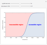 Temperature Dependence of Dehydrogenation of Ethyl Benzene to Styrene
Housam Binous -
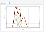 Deconvolution of a Chromatogram
Housam Binous -
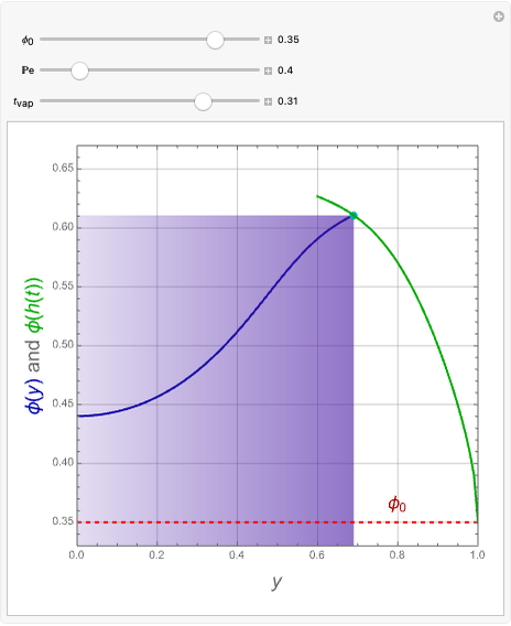 Distribution of Colloidal Particles during Solvent Evaporation
Housam Binous -
 Heat Conduction in a Rod
Housam Binous -
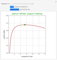
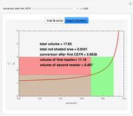 Optimal Setup of Two Continuous Stirred-Tank Reactors (CSTRs) in Series
Housam Binous -
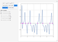
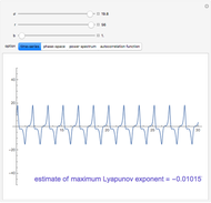 Study of the Dynamic Behavior of the Lorenz System
Housam Binous -
 A Graphically Enhanced Method for Computing Real Roots of Nonlinear Functions
Housam Binous -
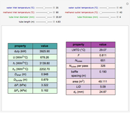 Design of a Shell and Tube Heat Exchanger
Housam Binous -
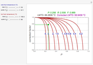 Correction Factor for Shell and Tube Heat Exchanger
Housam Binous -
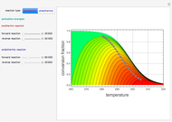 Contour Plots for Reaction Rates
Housam Binous -
 Optimal Conditions for CO2/n-Hexane Flash Separation
Housam Binous -
 Residual Functions for the SRK and PR Equations of State
Housam Binous -
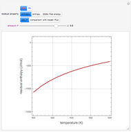
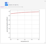 Gas-Phase Fugacity Coefficients for Propylene
Housam Binous -
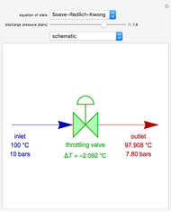 Operation of a Throttling Valve
Housam Binous -
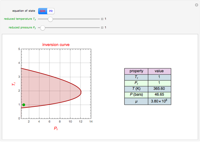 Joule-Thomson Inversion Curves for Soave-Redlich-Kwong (SRK) and Peng-Robinson (PR) Equations of State
Housam Binous -
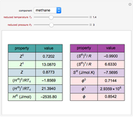 Lee-Kesler Generalized Correlations for Gases
Housam Binous -
 Mapping the Maxima for a Nonisothermal Chemical System
Housam Binous -
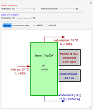 Operation of an Air Conditioner
Housam Binous -
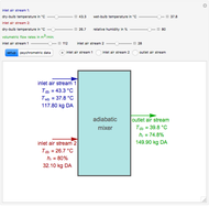 Adiabatic Mixing of Two Moist Air Streams
Housam Binous