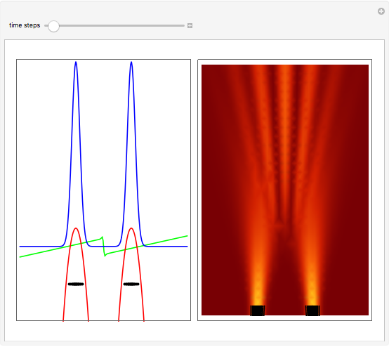
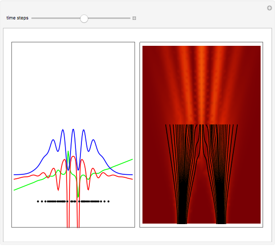
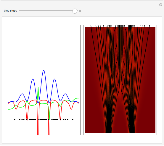
Causal Interpretation of the Double-Slit Experiment in Quantum Theory
Initializing live version


Requires a Wolfram Notebook System
Interact on desktop, mobile and cloud with the free Wolfram Player or other Wolfram Language products.
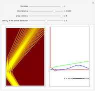
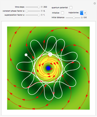
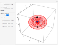
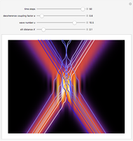
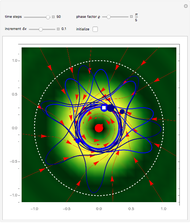
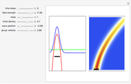
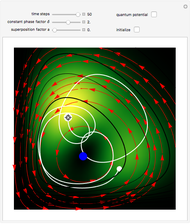
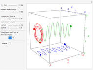
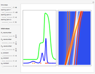
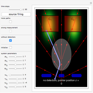
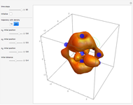
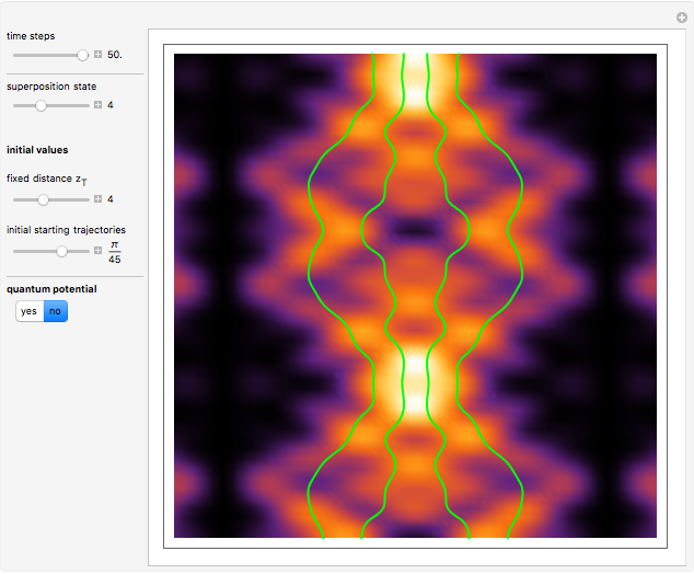
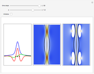
Probably one of the most interesting and fundamental wave-particle duality problems in modern physics is the double-slit experiment.
[more]


Contributed by: Klaus von Bloh (March 2011)
After work by: Chris Dewdney
Open content licensed under CC BY-NC-SA
Snapshots


Details
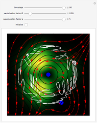
The trajectories were first numerically calculated in C. Philippidis, C. Dewdney, and B. J. Hiley, "Quantum Interference and the Quantum Potential," Il Nuovo Cimento 52B, 1979 pp. 15–28.
Permanent Citation
Related Demonstrations
More by Author
 Time-Dependent Scattering in the Causal Interpretation of Quantum Theory
Klaus von Bloh Radioactive Decay in the Causal Interpretation of Quantum Theory
Klaus von Bloh Simple Chaotic Motion of Quantum Particles According to the Causal Interpretation of Quantum Theory
Klaus von Bloh Causal Interpretation of the Free Quantum Particle
Klaus von Bloh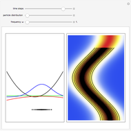 Causal Interpretation of the Quantum Harmonic Oscillator
Klaus von Bloh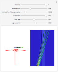 The Causal Interpretation of Quantum Tunneling through a Square Barrier and Well
Klaus von Bloh Influence of the Relative Phase in the de Broglie-Bohm Theory
Klaus von Bloh Double Delta Function Scattering Potential
Peter Falloon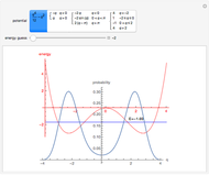 Quantum Well Explorer
Richard Gass Relativistic Quantum Dynamics in 1D and the Klein Paradox
Ulrich Mutze
-
 Bohm Trajectories for the Two-Dimensional Coulomb Potential
Klaus von Bloh -
 Bohm Trajectories in an LCAO Approximation for the Hydrogen Molecule H_2
Klaus von Bloh -
 Decoherence and Trajectories Implied by a Modified Schrodinger Equation
Klaus von Bloh -
 Bohm Trajectories for a Particle in a Two-Dimensional Circular Billiard
Klaus von Bloh -
 From Bohm to Classical Trajectories in a Hydrogen Atom
Klaus von Bloh -
 Continuous Transition between Quantum and Classical Behavior for a Harmonic Oscillator
Klaus von Bloh -
 Continuous Transition between Classical and Bohm Quantum Pictures for Young's Interference Experiment
Klaus von Bloh -
 Bohm Trajectories for Quantum Particles in a Uniform Gravitational Field
Klaus von Bloh -
 Bohm Trajectories for a Particle in a Two-Dimensional Calogero-Moser Potential
Klaus von Bloh -
 Nonlocality in the de Broglie-Bohm Interpretation of Quantum Mechanics
Klaus von Bloh -
 Three-Soliton Collision in the Trajectory Approach
Klaus von Bloh -
 The Which-Way Experiment and the Conditional Wavefunction
Klaus von Bloh -
 Chaotic Quantum Motion of Two Particles in a 3D Harmonic Oscillator Potential
Klaus von Bloh -
 Perturbation Theory in the de Broglie-Bohm Interpretation of Quantum Mechanics
Klaus von Bloh -
 Periodic Quantum Motion of Two Particles in a 3D Harmonic Oscillator Potential
Klaus von Bloh -
 Quantum Motion of Two Particles in a 3D Trigonometric Pöschl-Teller Potential
Klaus von Bloh -
 The Talbot Carpet in the Causal Interpretation of Quantum Mechanics
Klaus von Bloh -
 Bohmian Quantum Trajectories for Coherent States of the Pöschl-Teller Potential
Klaus von Bloh -
 Gray and Dark Solitons in the de Broglie and Bohm Approaches
Klaus von Bloh -
 A Breather Solution in the Causal Interpretation of Quantum Mechanics
Klaus von Bloh