Decoherence and Trajectories Implied by a Modified Schrodinger Equation


Requires a Wolfram Notebook System
Interact on desktop, mobile and cloud with the free Wolfram Player or other Wolfram Language products.
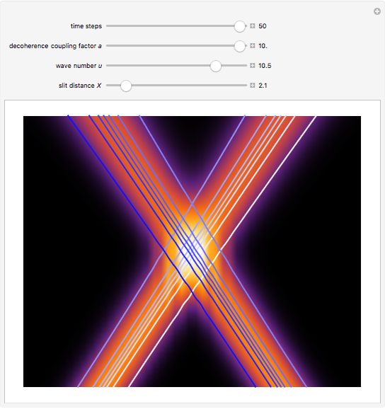
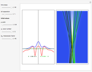
Decoherence is defined as the emergence of classical behavior through interaction of a quantum system with the environment. It is the most widely accepted explanation of how quantum systems become classical. For other points of view, see, for example, [1, 2]. Interference of coherent superposition of quantum amplitudes  ,
,  in Young's double-slit experiment is a preeminent feature of quantum systems, but in the classical limit, the interference term vanishes. Classical behavior is exhibited in the trajectories of the particles when each particle goes through one slit and is not affected by the other slit.
Contributed by: Partha Ghose and Klaus von Bloh (July 2017)
Open content licensed under CC BY-NC-SA
Snapshots

Details
The initial wavefunction in the eikonal form,
 ,
,
obeys the free-particle Schrödinger equation in the  direction:
 ,
,
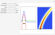
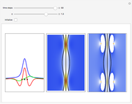
here with  . The initial wavefunction is a linear combination of two Gaussian packets with initial spatial half-widths
  and group velocities
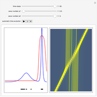
  . The measured intensity
  at any time
  is given by
 .
.
According to the theory proposed in [1], the measured intensity takes the form
 ,
,
with  and
and  , where
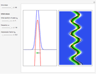
  is the coherence time, a measurement of how fast the system becomes classical. For simplicity,
  is called the decoherence coupling factor. In this context, classical means that the probability density
  becomes
 .
.
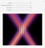
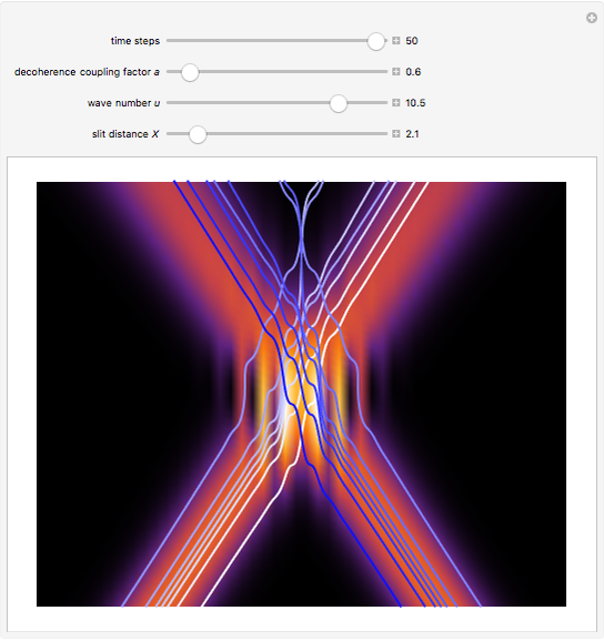
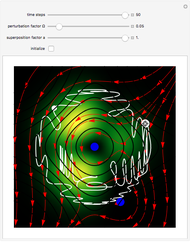
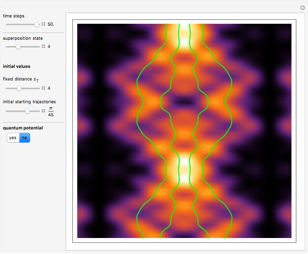
If  (the quantum limit), there is full coherence with
  and there is no difference between the general Bohm view and the quantum potential approach. The trajectories run to the local maxima of the squared wavefunction and therefore correspond to the bright fringes of the diffraction pattern. The quantum particle passes through slit one or slit two and never crosses the axis of symmetry.
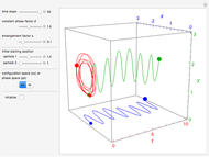
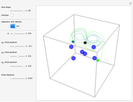
For unit mass  , the general equation of motion is given by the acceleration term that is the second derivative of the position
  with respect to time :
 ,
,
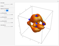
where is integrated numerically for various initial positions and velocities. The initial positions are linearly distributed around the peaks of the wave. The initial velocities are taken from the gradient of the phase function for  . The quantum potential
  , from which the trajectories are calculated, is given by:
 ,
,
with
 .
.
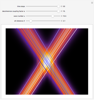
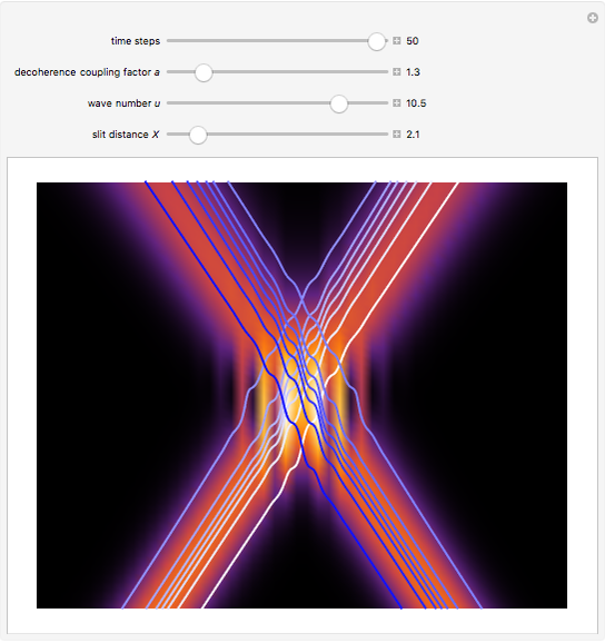
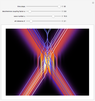
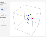
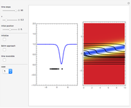
For  the coupling function
  , the effect of the quantum potential vanishes, and there is no dependence of the trajectories on the phase functions
  and
and  . This leads to the crossing of trajectories.
The results become more accurate if you increase AccuracyGoal, PrecisionGoal and MaxSteps.
For more detailed information about Bohmian mechanics, see [5, 6], and for an animated example describing a similar situation, see [7].
References
[1] P. Ghose, "Continuous Quantum-Classical Transitions and Measurement: A Relook." arxiv.org/abs/1705.09149v1.
[2] P. Ghose and K. von Bloh, "Continuous Transitions between Quantum and Classical Motions." arxiv.org/abs/1608.07963.
[3] A. S. Sanz and F. Borondo, "A Quantum Trajectory Description of Decoherence," The European Physical Journal D, 44(2), 2007 pp. 319–326. doi:10.1140/epjd/e2007-00191-8.
[4] B.-G. Englert, M. O. Scully, G. Süssman and H. Walther, "Surrealistic Bohm Trajectories," Zeitschrift für Naturforschung, 47(12), 1992 pp. 1175–1186. doi:10.1515/zna-1992-1201.
[5] "Bohmian-Mechanics.net." (Jun 29, 2017) www.bohmian-mechanics.net/index.html.
[6] S. Goldstein. "Bohmian Mechanics." The Stanford Encyclopedia of Philosophy. (Jun 29, 2017)plato.stanford.edu/entries/qm-bohm.
[7] P. Ghose and K. von Bloh. Decoherence and Crossing Trajectories in the de Broglie–Bohm Approach [Video]. (Jul 3, 2017), www.youtube.com/watch?v=ONw5SHIRe-0.
Permanent Citation
 Soliton Trajectories of the Modified Korteweg-de Vries Equation (mKdV)
Klaus von Bloh Bohm Trajectories for a Type of Derivative Nonlinear Schrödinger Equation
Klaus von Bloh Bohm Trajectories for a Particle in an Infinite 3D Box
Klaus von Bloh From Bohm to Classical Trajectories in a Hydrogen Atom
Partha Ghose and Klaus von Bloh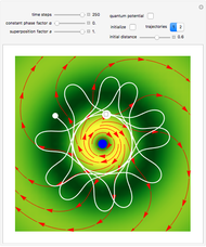 Bohm Trajectories for the Two-Dimensional Coulomb Potential
Klaus von Bloh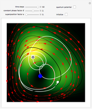 Bohm Trajectories for a Particle in a Two-Dimensional Calogero-Moser Potential
Klaus von Bloh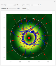 Bohm Trajectories for a Particle in a Two-Dimensional Circular Billiard
Klaus von Bloh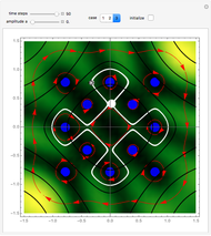 Bohmian Quantum Trajectories for Coherent States of the Pöschl-Teller Potential
Klaus von Bloh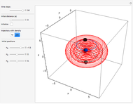 Bohm Trajectories in an LCAO Approximation for the Hydrogen Molecule H_2
Klaus von Bloh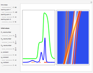 Three-Soliton Collision in the Trajectory Approach
Klaus von Bloh
-
Bohm Trajectories for the Two-Dimensional Coulomb Potential
Klaus von Bloh -
Bohm Trajectories in an LCAO Approximation for the Hydrogen Molecule H_2
Klaus von Bloh -
 Decoherence and Trajectories Implied by a Modified Schrodinger Equation
Klaus von Bloh -
Bohm Trajectories for a Particle in a Two-Dimensional Circular Billiard
Klaus von Bloh -
From Bohm to Classical Trajectories in a Hydrogen Atom
Klaus von Bloh -
 Continuous Transition between Quantum and Classical Behavior for a Harmonic Oscillator
Klaus von Bloh -
 Continuous Transition between Classical and Bohm Quantum Pictures for Young's Interference Experiment
Klaus von Bloh -
 Bohm Trajectories for Quantum Particles in a Uniform Gravitational Field
Klaus von Bloh -
Bohm Trajectories for a Particle in a Two-Dimensional Calogero-Moser Potential
Klaus von Bloh -
 Nonlocality in the de Broglie-Bohm Interpretation of Quantum Mechanics
Klaus von Bloh -
Three-Soliton Collision in the Trajectory Approach
Klaus von Bloh -
 The Which-Way Experiment and the Conditional Wavefunction
Klaus von Bloh -
 Chaotic Quantum Motion of Two Particles in a 3D Harmonic Oscillator Potential
Klaus von Bloh -
 Perturbation Theory in the de Broglie-Bohm Interpretation of Quantum Mechanics
Klaus von Bloh -
 Periodic Quantum Motion of Two Particles in a 3D Harmonic Oscillator Potential
Klaus von Bloh -
 Quantum Motion of Two Particles in a 3D Trigonometric Pöschl-Teller Potential
Klaus von Bloh -
 The Talbot Carpet in the Causal Interpretation of Quantum Mechanics
Klaus von Bloh -
Bohmian Quantum Trajectories for Coherent States of the Pöschl-Teller Potential
Klaus von Bloh -
 Gray and Dark Solitons in the de Broglie and Bohm Approaches
Klaus von Bloh -
 A Breather Solution in the Causal Interpretation of Quantum Mechanics
Klaus von Bloh