Three-Soliton Collision in the Trajectory Approach


Requires a Wolfram Notebook System
Interact on desktop, mobile and cloud with the free Wolfram Player or other Wolfram Language products.
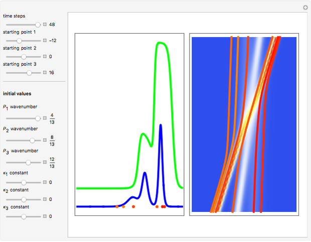
This Demonstration determines the streamlines or trajectories of idealized particles in a three-soliton collision, according to the Korteweg–de Vries equation (KdV) in  space. The collision of three solitons with different amplitudes involves the wave numbers
  ,
,  , and
, and  . These are, in turn, determined by the dispersion relations, given the speed of each wave. For the three-soliton system, the wave velocity depends on the amplitude. The constants
  ,
,  , and
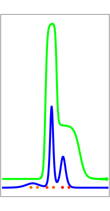
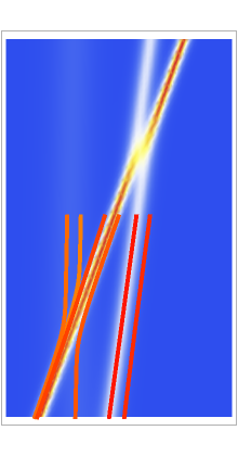
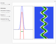
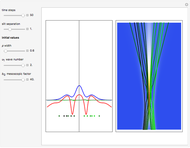
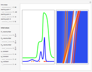
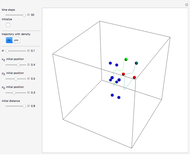
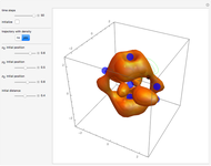
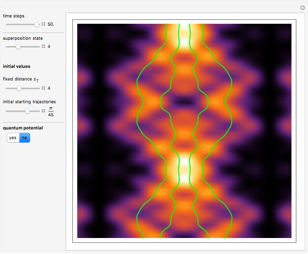
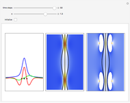
, and  determine the initial positions of the peaks of each soliton. The streamlines of the particles follow the current flow, which can be derived from the continuity equation. The concept of a trajectory is based on the causal interpretation of quantum mechanics developed by David Bohm. The three-soliton result is obtained by the Hirota direct method. The graphic on the left shows the density (blue) and the velocity (green) of the idealized particles. On the right, you can see the density and the trajectories in space.
Contributed by: Klaus von Bloh (January 2016)
Open content licensed under CC BY-NC-SA
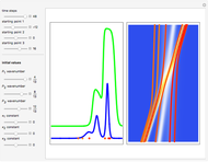
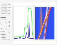
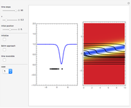
Snapshots


Details
In 1971 Hirota introduced a new direct method for constructing multi-soliton solutions to the integrable nonlinear Korteweg–de Vries equation  with the partial derivative
  and so on. The Hirota direct method makes a transformation to a bilinear equation via the transformation
  so that in the new form, the multi-soliton solutions can be solved using the Hirota
  -operator.
Specifically, the bilinear equation for the Korteweg–de Vries equation is
 ,
,
which can be solved by the Hirota -operator
 .
.
In the original work of Hirota, the KdV equation is solved using the ansatz
 ,
,
where the  matrix
  has the form
 ,
,
where  is the Kronecker delta and
  with the constant phase factor
  .
.
In practice, for the three-soliton, the  matrix is given by
 ,
,
where
 ,
,  ,
,  ,
,
 ,
,  , and
, and  .
.
The motion of the particles associated with the current flow can be extracted from the continuity equation  . The guiding equations depend only on the velocity, which for the KdV equation become
  .
.
With the transformation the velocity term, which is also bilinear, is
 .
.
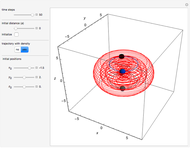
The starting points of possible trajectories inside the wave can be chosen by the settings  ,
,  , and
, and  . The initial points should be distributed around the peak of each wave. The single trajectories are calculated using
  . The system is time reversible:
  . Due to the singularities, the size of the velocity term, and computational limitations, the wave numbers
  have to be chosen carefully.
References
[1] R. Hirota, "Exact Solution of the Korteweg–de Vries Equation for Multiple Collisions of Solitons," Physical Review Letters, 27(18), 1971 pp. 1192–1194. doi:10.1103/PhysRevLett.27.1192.
[2] "Bohmian-Mechanics.net." (Jan 6, 2015) www.bohmian-mechanics.net/index.html.
[3] S. Goldstein. "Bohmian Mechanics." The Stanford Encyclopedia of Philosophy. (Mar 4, 2013)plato.stanford.edu/entries/qm-bohm.
Permanent Citation
 Gray and Dark Solitons in the de Broglie and Bohm Approaches
Klaus von Bloh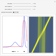 Soliton Trajectories of the Modified Korteweg-de Vries Equation (mKdV)
Klaus von Bloh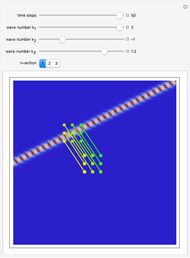 Soliton Trajectories for the Kadomtsev-Petviashvili Equation
Klaus von Bloh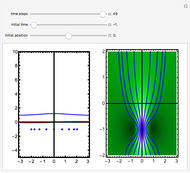 Peregrine Soliton with Controllable Center in the Causal Interpretation of Quantum Mechanics
Klaus von Bloh Bohm Trajectories for a Particle in an Infinite 3D Box
Klaus von Bloh Decoherence and Trajectories Implied by a Modified Schrodinger Equation
Partha Ghose and Klaus von Bloh From Bohm to Classical Trajectories in a Hydrogen Atom
Partha Ghose and Klaus von Bloh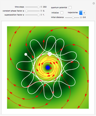 Bohm Trajectories for the Two-Dimensional Coulomb Potential
Klaus von Bloh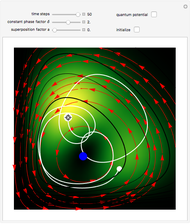 Bohm Trajectories for a Particle in a Two-Dimensional Calogero-Moser Potential
Klaus von Bloh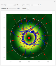 Bohm Trajectories for a Particle in a Two-Dimensional Circular Billiard
Klaus von Bloh
-
Bohm Trajectories for the Two-Dimensional Coulomb Potential
Klaus von Bloh -
 Bohm Trajectories in an LCAO Approximation for the Hydrogen Molecule H_2
Klaus von Bloh -
Decoherence and Trajectories Implied by a Modified Schrodinger Equation
Klaus von Bloh -
Bohm Trajectories for a Particle in a Two-Dimensional Circular Billiard
Klaus von Bloh -
From Bohm to Classical Trajectories in a Hydrogen Atom
Klaus von Bloh -
 Continuous Transition between Quantum and Classical Behavior for a Harmonic Oscillator
Klaus von Bloh -
 Continuous Transition between Classical and Bohm Quantum Pictures for Young's Interference Experiment
Klaus von Bloh -
 Bohm Trajectories for Quantum Particles in a Uniform Gravitational Field
Klaus von Bloh -
Bohm Trajectories for a Particle in a Two-Dimensional Calogero-Moser Potential
Klaus von Bloh -
 Nonlocality in the de Broglie-Bohm Interpretation of Quantum Mechanics
Klaus von Bloh -
 Three-Soliton Collision in the Trajectory Approach
Klaus von Bloh -
 The Which-Way Experiment and the Conditional Wavefunction
Klaus von Bloh -
 Chaotic Quantum Motion of Two Particles in a 3D Harmonic Oscillator Potential
Klaus von Bloh -
 Perturbation Theory in the de Broglie-Bohm Interpretation of Quantum Mechanics
Klaus von Bloh -
 Periodic Quantum Motion of Two Particles in a 3D Harmonic Oscillator Potential
Klaus von Bloh -
 Quantum Motion of Two Particles in a 3D Trigonometric Pöschl-Teller Potential
Klaus von Bloh -
 The Talbot Carpet in the Causal Interpretation of Quantum Mechanics
Klaus von Bloh -
 Bohmian Quantum Trajectories for Coherent States of the Pöschl-Teller Potential
Klaus von Bloh -
Gray and Dark Solitons in the de Broglie and Bohm Approaches
Klaus von Bloh -
 A Breather Solution in the Causal Interpretation of Quantum Mechanics
Klaus von Bloh