Convergence of Binomial Option Pricing under Nonconstant Volatility

Requires a Wolfram Notebook System
Interact on desktop, mobile and cloud with the free Wolfram Player or other Wolfram Language products.
This Demonstration is a continuation and test of the validity of a modeling approach presented by the Wolfram Demonstration European Binomial Option Pricing with Nonconstant Volatility. That Demonstration presents a model for pricing an option using binomial option pricing techniques when volatility of the underlying asset is not deemed to be constant through time.
[more]


Contributed by: Tom Stannard (November 2015)
Open content licensed under CC BY-NC-SA
Snapshots

Details
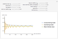
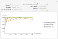
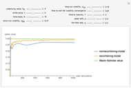
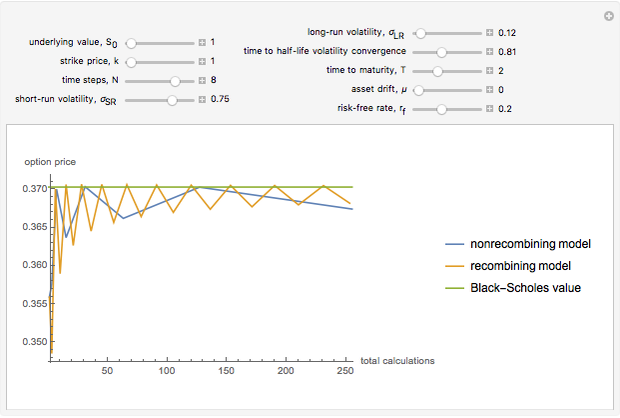
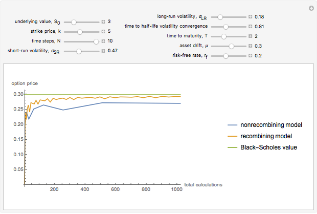
When you choose the number of time steps, the Demonstration calculates expected values from the models for that number of time steps and each number of time steps preceding it.
The number of time steps you set relates only to the nonrecombining approach. Once chosen, the total number of calculations needed to calculate the value is found. In the nonrecombining case, there are  calculations after all the possible prices have been calculated and maximums taken at the terminal nodes (i.e., once the process for the underlying value has been estimated using the binomial tree).
Following this, the total number of calculations is used to solve how many time steps the recombining approach would use to match that number of total calculations. For instance, if  is chosen to be
  , there are
  calculations required by the nonrecombining approach. The Demonstration takes
  and solves
  for (the total number of calculations for the recombining approach given time steps). In this case, the closest number of time steps that yields this number of calculations is
  (giving
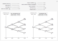
  total calculations). Therefore, when the nonrecombining approach is set at time steps (and the Demonstration depicts expected value calculations), the recombining approach will be set at time steps and depict expected value calculations. This is done simply to enhance the visual descriptiveness of the Demonstration.
For the estimation of the Black–Scholes value, note that we cannot estimate the volatility for the process of the underlying asset through time as it is not constant (that is, we cannot directly estimate the process for  ). However, we can estimate the distribution of
  (the terminal value; see [3]). This means that we can calculate a volatility of the terminal value of the underlying asset. The volatility calculation in the original Demonstration after
  moves is:
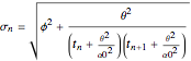 .
.
For the Black–Scholes estimation this simply reduces to:
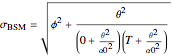 .
.
References
[1] G. Guthrie, "Learning Options and Binomial Trees," Wilmott Journal: The International Journal of Innovative Quantitative Finance Research, 3(1), 2011 pp. 1–23. doi:10.1002/wilj.42.
[2] J. C. Cox, S. A. Ross, and M. Rubinstein, "Option Pricing: A Simplified Approach," Journal of Financial Economics, 7(3), 1979 pp. 229–263. doi:10.1016/0304-405X(79)90015-1.
[3] J. C. Hull, Options, Futures, and Other Derivatives, 8th ed., Boston: Prentice Hall, 2012.
Permanent Citation
 European Binomial Option Pricing with Nonconstant Volatility
Tom Stannard and Graeme Guthrie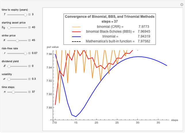 Convergence of Binomial, Binomial Black-Scholes, and Trinomial Option Pricing Methods
Michail Bozoudis Binomial Option Pricing Model
Fiona Maclachlan Nonuniqueness of Option Pricing Under the Meixner Model
Andrzej Kozlowski Pricing Put Options with the Binomial Method
Michail Bozoudis Option Prices under the Fractional Black-Scholes Model
Andrzej Kozlowski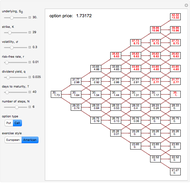 Trinomial Tree Option Pricing Method
Darius Kirevicius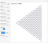 Adaptive Mesh Trinomial Tree for Vanilla Option Pricing
Darius Kirevicius Barrier Option Pricing within the Black-Scholes Model
Peter Falloon Binary Options: Pricing and Greeks
Peter Falloon
-
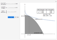 General Equilibrium with Production: Robinson Crusoe with and without Trade
Tom Stannard -
 Convergence of Binomial Option Pricing under Nonconstant Volatility
Tom Stannard -
European Binomial Option Pricing with Nonconstant Volatility
Tom Stannard -
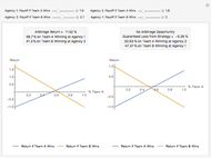 Sports Arbitrage: Two-Agency, Two-Outcome Efficient Pricing Test
Tom Stannard