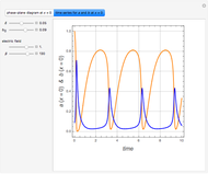
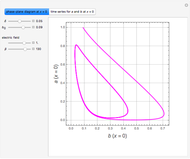
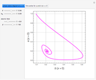
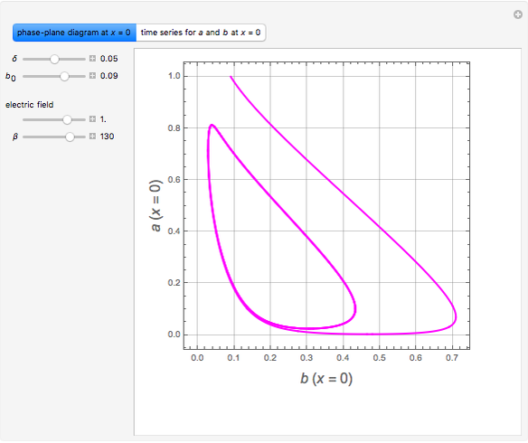
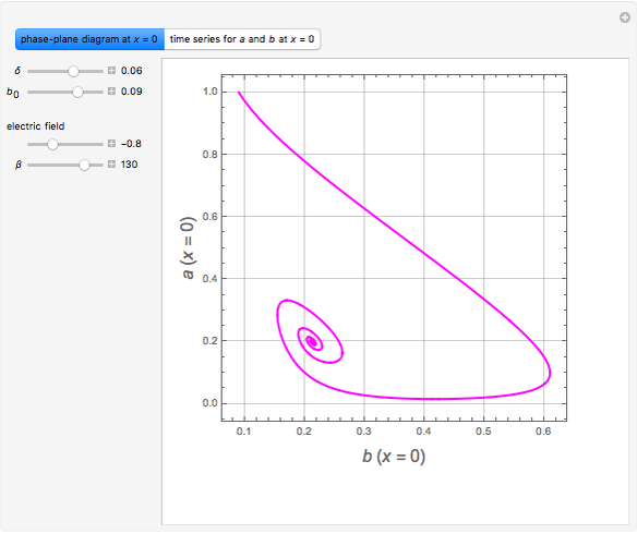
Gray-Scott Reaction-Diffusion Cell with an Applied Electric Field


Requires a Wolfram Notebook System
Interact on desktop, mobile and cloud with the free Wolfram Player or other Wolfram Language products.
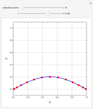
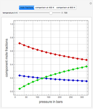
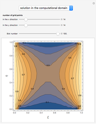
Consider the Gray–Scott reaction-diffusion cell with an applied electric field. The governing equations and boundary and initial conditions are:
[more]


Contributed by: Housam Binousand Brian G. Higgins (June 2013)
Open content licensed under CC BY-NC-SA
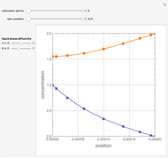
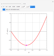
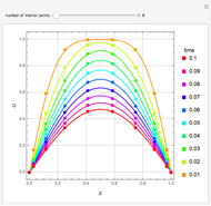
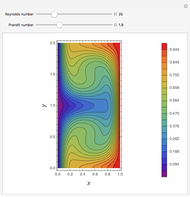
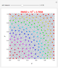
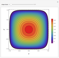
Snapshots

Details
In the discrete Chebyshev–Gauss–Lobatto case, the interior points are given by  . These points are the extrema of the Chebyshev polynomials of the first kind,
  .
.
The  Chebyshev derivative matrix at the quadrature points is an matrix
  given by
 ,
,  ,
,  for
for  , and
, and  for
for  and
and  ,
,
where  for and
  .
.
The matrix  is then used as follows:
  and
and  , where
  is a vector formed by evaluating
  at
at  ,
,  , and
, and  and
and  are the approximations of
  and
and  at the .
Reference
[1] P. Moin, Fundamentals of Engineering Numerical Analysis, Cambridge, UK: Cambridge University Press, 2001.
[2] L. N. Trefethen, Spectral Methods in Matlab, Philadelphia: SIAM, 2000.
[3] A. W. Thornton and T. R. Marchant, "Semi-analytical solutions for a Gray–Scott reaction–diffusion cell with an applied electric field," Chemical Engineering Science, 63(2), 2008 pp. 495–502. DOI: 10.1016/j.ces.2007.10.001 .
Permanent Citation
 Second-Order Reaction with Diffusion in a Liquid Film
Housam Binous and Brian G. Higgins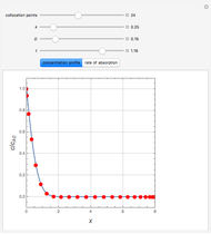 Absorption with Chemical Reaction in a Semi-Infinite Medium
Housam Binous and Brian G. Higgins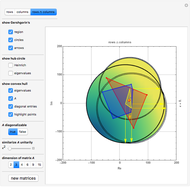 Enclosing the Spectrum by Gershgorin-Type Sets
Ludwig Weingarten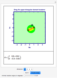 Numerical Range for Some Complex Upper Triangular Matrices
Ludwig Weingarten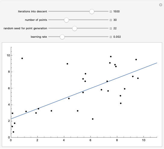 Linear Regression with Gradient Descent
Jonathan Kogan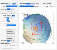 Brauer's Cassini Ovals versus Gershgorin Circles
Ludwig Weingarten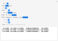 Solving Matrix Systems with Real, Interval, or Uncertain Elements
Valter Yoshihiko Aibe and Mikhail Dimitrov Mikhailov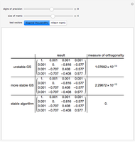 Numerical Instability in the Gram-Schmidt Algorithm
Chris Boucher Solving a Linear System with Uncertain Coefficients
Valter Yoshihiko Aibe and Mikhail Dimitrov Mikhailov Maximum Absolute Column Sum Norm
Eugenio Bravo Sevilla
-
 Distribution of Colloidal Particles during Solvent Evaporation
Brian G. Higgins -
 Heat Conduction in a Rod
Brian G. Higgins -
 A Graphically Enhanced Method for Computing Real Roots of Nonlinear Functions
Brian G. Higgins -
 All Real Roots of a Nonlinear System of Equations
Brian G. Higgins -
 Seader's Method for Real Roots of a Nonlinear Equation
Brian G. Higgins -
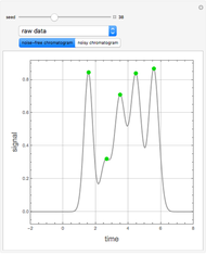 Analysis of Chromatographic Data
Brian G. Higgins -
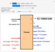 Combustion Reactions in a Furnace
Brian G. Higgins -
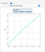 Boundary Value Problem Using Galerkin's Method
Brian G. Higgins -
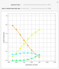 Operation of an Ethane Steam Cracker
Brian G. Higgins -
 Gibbs Free Energy Minimization Applied to the Haber Process
Brian G. Higgins -
 Minimum of a Function Using the Fibonacci Sequence
Brian G. Higgins -
 Transient Heat Conduction Using Chebyshev Collocation
Brian G. Higgins -
 Steady-State Two-Dimensional Convection-Diffusion Equation
Brian G. Higgins -
 Peak Retention Time Using Discrete Fourier Transform
Brian G. Higgins -
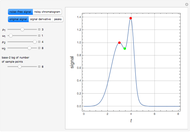
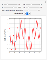 First and Second Derivatives of a Periodic Function Using Discrete Fourier Transforms
Brian G. Higgins -
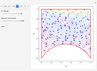 Stokes Flow in Container with Concave Bottom
Brian G. Higgins -
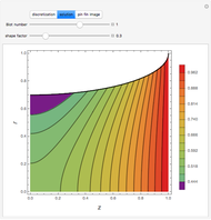 Cooling with a Shaped Pin Fin
Brian G. Higgins -
 Solution of the Laplace Equation Using Coordinates Fitted to the Boundary Conditions
Brian G. Higgins -
 Flow Through a Rectangular Duct
Brian G. Higgins -
 Flow through Chamfered Ducts
Brian G. Higgins