Lagrange Multipliers in Two Dimensions


Requires a Wolfram Notebook System
Interact on desktop, mobile and cloud with the free Wolfram Player or other Wolfram Language products.
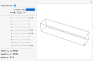
This Demonstration intends to show how Lagrange multipliers work in two dimensions.
[more]
Contributed by: Cedric Voisin (July 2012)
Open content licensed under CC BY-NC-SA
Snapshots


Details
The function  (plotted in red) is the one to be optimized subject to the constraint. Here
 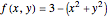 . The function
  is the constraint function, plotted in blue. The constraint is its particular contour line
  . Here
  , so the constraint is
  , which is simpler to visualize (thick blue line). In this particular case, the new potential
  is a Legendre transformation, where
  (given the constraint ). Hence, as
  , for obvious symmetry reasons the complete solution here is quite simple:
 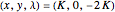 . The function
  (plotted in green) is the difference in height between
  and the rescaled constraint function
  , which is constant only when and are parallel. The equilibrium condition
  (
( ) can be seen as a constraint on
  .
.
The main ideas behind the Lagrange multipliers have already been discussed in the 1D case. See Lagrange Multipliers in One Dimension.
This Demonstration illustrates the 2D case, where in particular, the Lagrange multiplier is shown to modify not only the relative slopes of the function to be minimized and the rescaled constraint (which was already shown in the 1D case), but also their relative orientations (which do not exist in the 1D case).
This in turn shows how the independence of  and
and  is restored by the introduction of (which is adjusted so that and are strictly parallel in both slope and orientation, so that their height difference remains constant near the solution, with no more constraint between and ).
The global problem can be understood as finding a point that is:
1. on the particular contour line , and
2. on a contour line  or
or  (the constant is unknown, as the contour line is what we are looking for) tangent to the previous one.
By imposing  (for any ), we impose that and
  share the same orientation but with different relative slopes (depending on ).
is then a tuning tool to find the place where the functions and have the same slope (strict parallelism) and hence where the potential  is an extremum (equilibrium situation).
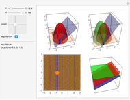
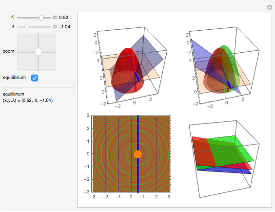
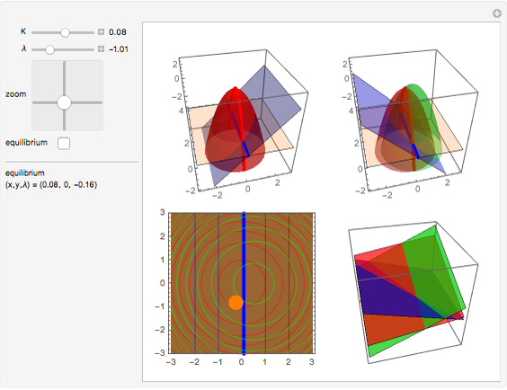
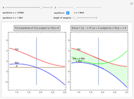
Here are a few explanations for each of the four plots displayed:
• upper-left: this is the case treated without the Lagrange multiplier. The thick blue line is the constraint, the thick red line is its projection on , and the solution is the top of the red thick line.
• upper-right: this is the case treated with the help of . The constraint function  is rescaled (), but as
  , the constraint (thick blue line) keeps the same position as in the previous case. The function plotted in green is the new potential, which is to be optimized without constraint on
  . When equilibrium is forced, its extremum corresponds to the solution of the problem. When equilibrium is not forced, it is a function of the three variables , , .
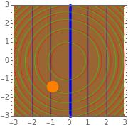
• bottom-left: same as upper-right, but with a contour representation, which shows more clearly the contour lines and the extremums of the three functions involved. The orange point is the one given by the 2D slider. When equilibrium is forced, it shows the solution of the problem (top of the green function ); otherwise it can be used to explore the slopes with the bottom-right panel.
• bottom-right: this is a close-up (tangent planes) of the plots of the three functions involved around the position (orange point) chosen by the 2D slider. It allows a comparison between their slopes. In particular, when , and have the same orientation but different slopes (this amounts to the 1D problem), and near the solution, they become completely parallel. When  , their orientations are different. When equilibrium is forced, their slopes remain parallel, hence remains horizontal (constant).
When forcing equilibrium, you can only change  (then , , and are the computed unique solution of the problem).
With the equilibrium box unchecked, you can change (a slider) and (2D slider) to get a feeling of how they act and what they mean.
Permanent Citation
 Lagrange Multipliers in One Dimension
Cedric Voisin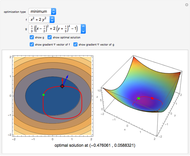 Constrained Optimization
Edda Eich-Soellner (University of Applied Sciences, München, Germany)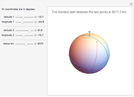 Shortest Path between Two Points on a Sphere
Bernard Vuilleumier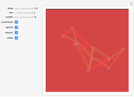 Constrained Optimal Routes in 3D Space
Vitaliy Kaurov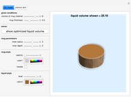 The Mug That Holds the Most Liquid
Frederick Wu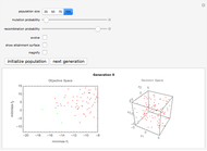 Evolutionary Multiobjective Optimization
Robin Gruna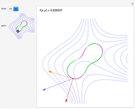 The Geometry of Lagrange Multipliers
Michael Rogers (Oxford College of Emory University) Geometric Representation of Method of Lagrange Multipliers
Shashi Sathyanarayana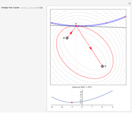 Lagrange's Milkmaid Problem
Erik Mahieu Shortest Path between Two Points in the Unit Disk Reflecting off the Circumference
Jingang Shi and Aaron T. Becker
-
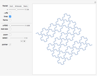 Continuous Changes in Self-Similar Fractals
Cedric Voisin -
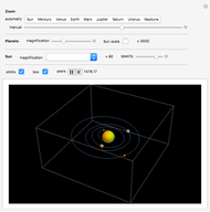 Length Scales in the Solar System
Cedric Voisin -
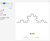 Parametrization of a Fractal Curve
Cedric Voisin -
 Lagrange Multipliers in Two Dimensions
Cedric Voisin -
Lagrange Multipliers in One Dimension
Cedric Voisin -
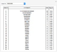 Logarithm Seen as the Size of a Number
Cedric Voisin -
 A Complex Wave in One Dimension
Cedric Voisin -
 A 1D Random Walk with Fractal Dimension 2.0
Cedric Voisin -
 Derivative of log(x!)
Cedric Voisin -
 Note Positions on a Violin
Cedric Voisin -
 Random Natural 3D tree
Cedric Voisin