Time Series for Power-Law Decay


Requires a Wolfram Notebook System
Interact on desktop, mobile and cloud with the free Wolfram Player or other Wolfram Language products.
Power-law decay time series are characterized by autocorrelation functions that decay as  , where
  is the lag and
  is the decay parameter. When
  , the time series exhibits strong persistence, with smaller values of
  indicating stronger persistence. When
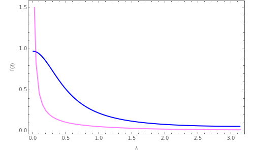
  , the time series exhibits high-frequency (or alternating) behavior and is said to be anti-persistent. Such time series are also characterized by a spectral density function that is proportional to
  , where
  is the radial frequency.

Contributed by: Justin Veenstra and Ian McLeod (November 2012)
(Western University)
Open content licensed under CC BY-NC-SA
Snapshots

Details
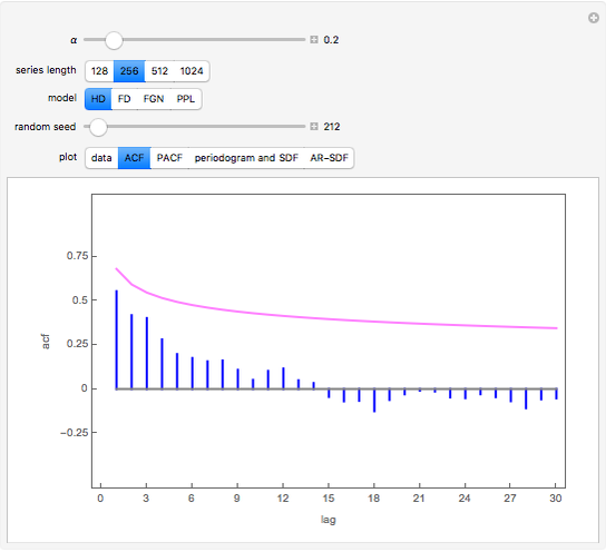
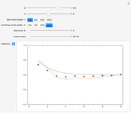
Snapshot 1: This shows the autocorrelation for FGN with  and series length
  . The setting corresponds to a Hurst coefficient of 0.9, which indicates very strong persistence. We see there is a large bias in the usual sample autocorrelation, since the true value is always much larger, except at lag 1.
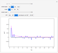
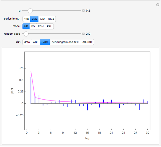
Snapshot 2: This shows the partial autocorrelation for the same data used in snapshot 1. The partial autocorrelation was estimated using the Burg algorithm, and it seems to do a better job.
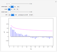
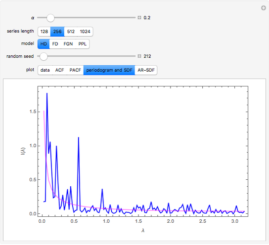
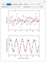
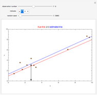
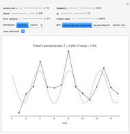
Snapshot 3: The periodogram and its expected value, the SDF, are shown.
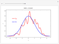
Snapshot 4: The SDF is shown in magenta along with its estimate in blue. The SDF is estimated by fitting an AR model using the Burg algorithm with model order determined using the AIC criterion.
For an overview and further references for the time series models, see [1].
Reference
[1] J. Q. Veenstra and A. I. McLeod, "A New Hyperbolic Decay Time Series Model," 2012. Submitted for publication.
Permanent Citation
 Aliasing in Time Series Analysis
Ian McLeod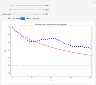 Tempered Fractionally Differenced White Noise
Ian McLeod, Mark Meerschaert and Farzad Sabzikar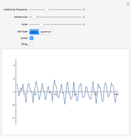 Frequency Spectrum of a Noisy Signal
Jon McLoone Wireless Power Transmission
Y. Shibuya Energy and Power of Signals
Daniel de Souza Carvalho Time Shifting and Time Scaling in Signal Processing
Aaron T. Becker and Mable Wan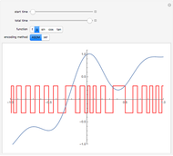 Time Encoding of Analog Signals
Andre Kessler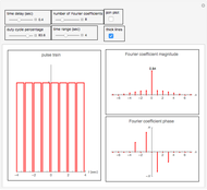 Fourier Series Coefficients of a Rectangular Pulse Signal
Nasser M. Abbasi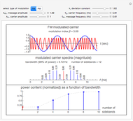 Power Content of Frequency Modulation and Phase Modulation
Nasser M. Abbasi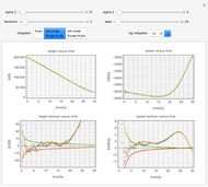 Tuning an Extended Kalman Filter
Brian C. Beckman
-
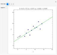 Anscombe Quartet
author -
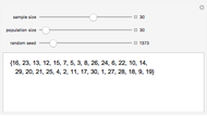 Random Samples and Random Permutations
author -
 Principal Components
author -
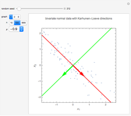
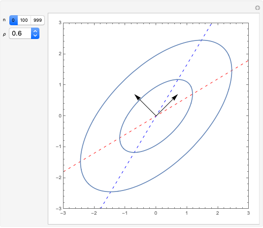
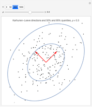 Karhunen-Loeve Directions
author -
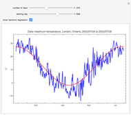 Plotting a Long Time Series
author -
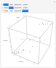 Visualizing Higher-Dimensional Data with 3D Scatterplots
author -
 Karhunen-Loeve Directions and Regression
author -
 Rank Transform in Harmonic Regression Time Series
author -
 Block Bootstrap for Time Series
author -
 Fractional Gaussian Noise
author -
 Mean, Fitted-Value, Error, and Residual in Simple Linear Regression
author -
 Simulated Coin Tossing Experiments and the Law of Large Numbers
author -
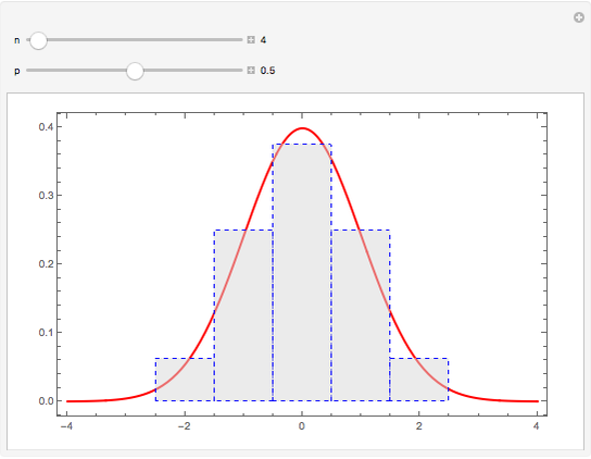 Illustrating the Central Limit Theorem with Sums of Bernoulli Random Variables
author -
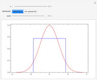 Illustrating the Central Limit Theorem with Sums of Uniform and Exponential Random Variables
author -
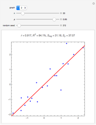 Visualizing R-Squared in Statistics
author -
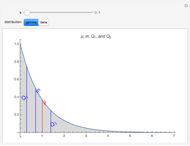 Mean, Median, and Quartiles in Skewed Distributions
author -
 Standard Normal Distribution Areas
author -
 Variance-Bias Tradeoff
author -
Aliasing in Time Series Analysis
author -
 Detecting Periodicity in Short Time Series
author