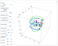
Bohm Trajectories for the Anisotropic Coulomb Potential with Constant Phase Shift

Requires a Wolfram Notebook System
Interact on desktop, mobile and cloud with the free Wolfram Player or other Wolfram Language products.
In the nonrelativistic de Broglie–Bohm approach, the electron in a hydrogen-like atom is not moving in the stationary  state. More generally, this is true when the phase function does not depend on the spatial coordinates or when the wavefunction is a real-valued function. For the hydrogen-like atom in an eigenstate, the electron can be considered to be in motion if the magnetic quantum number
  . The quantum particle orbits the
  axis in a circle of constant radius
  (for more details see [1]). In most other cases, any superposition state leads to a moving electron.


Contributed by: Klaus von Bloh (June 13)
Open content licensed under CC BY-NC-SA
Details
The three-dimensional stationary Schrödinger equation with Coulomb potential  can be written in parabolic coordinates
  as
as
 ,
,
with the wavefunction  , the Laplace operator
  , the partial derivative
  with respect to time and the Coulomb potential
  . For simplicity, we set atomic units
  .
.
In spherical polar coordinates, the unnormalized energy eigenfunctions for the hydrogen atom associated with the quantum state with the quantum numbers  is given by:
 ,
,
where  is a spherical harmonic. The radial function is
 ,
,
where  is a generalized Laguerre polynomial.
For a stationary case with  , the phase function
  reduces to zero. Thus the Bohm momentum
  of the ground state electron is
  , and finally the electron is at rest [1]. For
  , the electron is in motion.
If the wavefunction is expressed in parabolic coordinates (for more details see [4–6]), we find:
 ,
,
where
 ,
,
 ,
,
 .
.
Here  ,
,  and
and  is a Whittaker function.
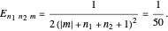
The energy spectrum depends only on the integers  ,
,  and
and  .
.
For the anisotropic Coulomb potential, the Schrödinger equation in Cartesian coordinates is:
with
 ,
,
and so on.
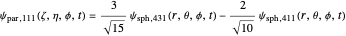
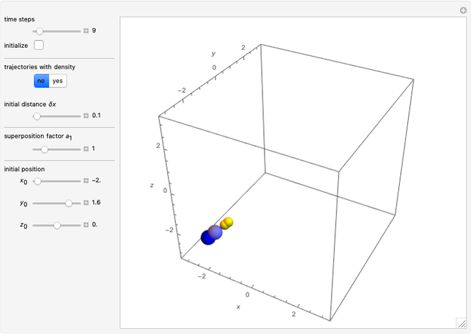
Due to computational limitations, the superposed total wavefunctions  are taken as a sum of just three eigenfunctions
  , where the unnormalized wavefunction
  for a particle is written as:
 ,
,
with  and (here,
  ).
).
Each part of the superposition of the three stationary state has the same energy:
The parabolic wavefunction  could be expressed by a linear combination of stationary states of spherical wavefunction
  . For example,
 .
.
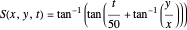
Let  for convenience. After variable transformations from parabolic coordinates to Cartesian coordinates, we obtain the total phase function
  :
:
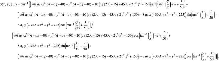
The gradient of the phase  is obtained from the total wavefunction in polar form,
  , with the quantum amplitude
  . The velocity field
  is calculated by the Bohm momentum
  with mass
  . From the Bohm momentum
  it follows that

(here,  ).
).
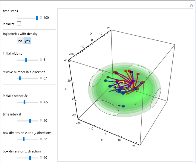
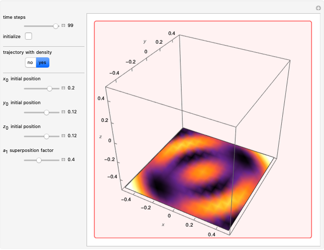
In the case of the superposition of the three stationary states with equal energy, the corresponding differential equation system for the velocity field becomes autonomous and obeys the time-independent part of the continuity equation  with the wave density
  .
.
For  the wavefunction
  in parabolic coordinates reduces to
  ,
,
with the total phase function  :
:
 .
.
This could be simplified for  :
:
 .
.
The trajectories reduce to circles with the velocities:
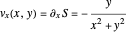 ,
,
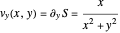
and
 .
.
The velocity depends on the position of the particle only. For  and
and  , most of the orbits form "spirally circles" along the
  axis, in which a spiral orbit is perpendicular on the circle orbit (for an example, see [7]).
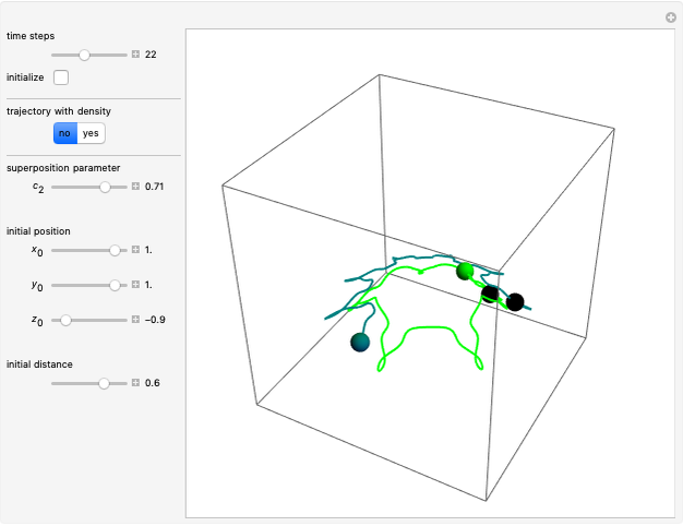
In all other cases, the integration of the velocity vector  in respect to time leads to complex periodic or chaotic orbits (for examples, see [8, 9]). If
  with
with  (
( ), it is strongly implied that chaotic motion occurs.
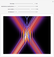
 When PlotPoints, AccuracyGoal, PrecisionGoal and MaxSteps are increased (if enabled), the results will be more accurate.
References
[1] P. R. Holland, The Quantum Theory of Motion: An Account of the de Broglie–Bohm Causal Interpretation of Quantum Mechanics, New York: Cambridge University Press, 1993.
[2] Bohmian-Mechanics.net. (Dec 26, 2022) bohmian-mechanics.net.
[3] S. Goldstein, "Bohmian Mechanics." The Stanford Encyclopedia of Philosophy (Summer 2017 Edition). (Dec 26, 2022) plato.stanford.edu/entries/qm-bohm.
[4] L. I. Schiff, Quantum Mechanics, 2nd ed., New York: McGraw-Hill, 1955.
[5] E. Merzbacher, Quantum Mechanics, New York: Wiley, 1961.
[6] J. F. Ogilvie, "The Hydrogen Atom According to Wave Mechanics: Part II. Paraboloidal Coordinates," Revista de Ciencia y Tecnologia, 32(2), 2016 pp. 25–39. arXiv:1612.05098.
[7] K. von Bloh. Bohm Trajectories for the Anisotropic Coulomb Potential with Constant Phase Shift: Part 3 [Video]. (Dec 28, 2022) www.youtube.com/watch?v=kIxbf256IlE.
[8] K. von Bloh. Bohm Trajectories for the Anisotropic Coulomb Potential in Parabolic Coordinates: Part 1 [Video]. (Dec 26, 2022) www.youtube.com/watch?v=mhkX1VArlT0.
[9] K. von Bloh. Bohm Trajectories for the Anisotropic Coulomb Potential with Constant Phase Shift: Part 2 [Video]. (Dec 26, 2022) www.youtube.com/watch?v=mmNFFvksa8Q.
Snapshots


Permanent Citation
 Bohm Trajectories for the Two-Dimensional Coulomb Potential
Klaus von Bloh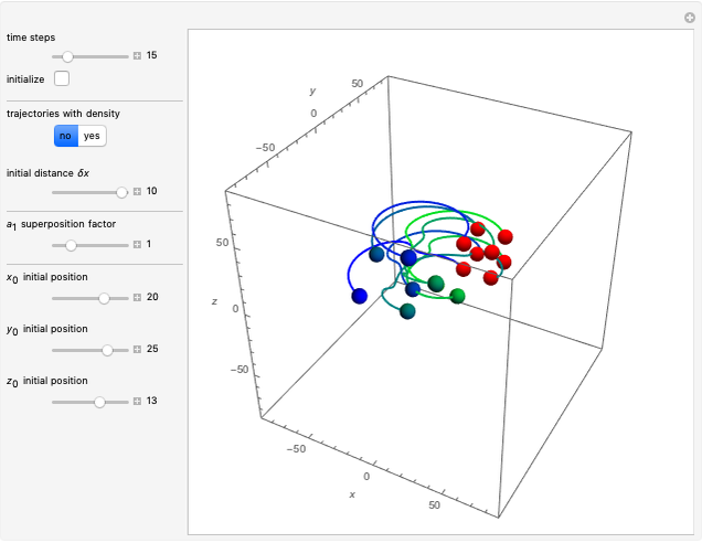 Bohm Trajectories for the Noncentral Hartmann Potential
Klaus von Bloh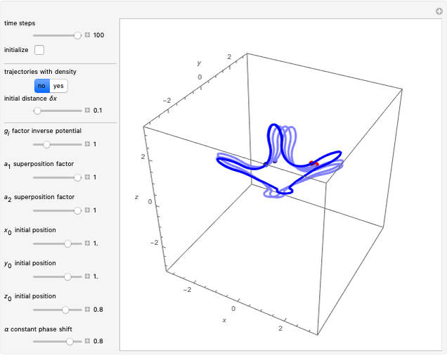 Bohm Trajectories for a Special Type of a Pseudoharmonic Potential
Klaus von Bloh Bohm Trajectories for an Isotropic Harmonic Oscillator with Added Inverse Quadratic Potential
Klaus von Bloh From Bohm to Classical Trajectories in a Hydrogen Atom
Partha Ghose and Klaus von Bloh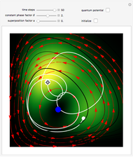 Bohm Trajectories for a Particle in a Two-Dimensional Calogero-Moser Potential
Klaus von Bloh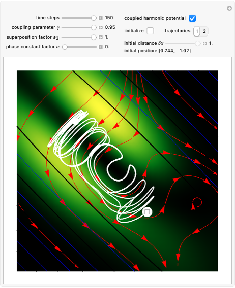 Bohm Trajectories for a Coupled Two-Dimensional Harmonic Oscillator
Klaus von Bloh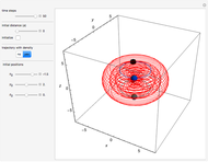 Bohm Trajectories in an LCAO Approximation for the Hydrogen Molecule H_2
Klaus von Bloh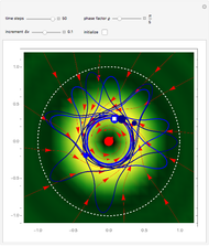 Bohm Trajectories for a Particle in a Two-Dimensional Circular Billiard
Klaus von Bloh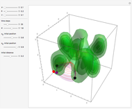 Bohm Trajectories for a Particle in an Infinite 3D Box
Klaus von Bloh
-
 The Superposition Principle in the Causal Interpretation of Quantum Mechanics
Klaus von Bloh -
Bohm Trajectories for a Coupled Two-Dimensional Harmonic Oscillator
Klaus von Bloh -
 Bohm Trajectories for the Anisotropic Coulomb Potential with Constant Phase Shift
Klaus von Bloh -
 The Double-Slit Experiment in a Uniform Potential
Klaus von Bloh -
 Two Rotating Waves in de Broglie-Bohm Mechanics
Klaus von Bloh -
 The Rotating Wave in de Broglie-Bohm Mechanics
Klaus von Bloh -
 The Three-Dimensional Isotonic Potential in Bohmian Mechanics
Klaus von Bloh -
 Ontology of the One-Dimensional Wavefunction in Bohmian Mechanics
Klaus von Bloh -
Bohm Trajectories for the Noncentral Hartmann Potential
Klaus von Bloh -
Bohm Trajectories for a Special Type of a Pseudoharmonic Potential
Klaus von Bloh -
 Collision of Two Neutrons in the de Broglie?Bohm Approach
Klaus von Bloh -
 Quantum Motion in an Infinite Spherical Well
Klaus von Bloh -
 The sp Hybrid Orbital in Bohmian Mechanics
Klaus von Bloh -
 Quantum Orbits of a Particle in Spherical Coordinates in a Three-Dimensional Harmonic Oscillator Potential
Klaus von Bloh -
Bohm Trajectories for an Isotropic Harmonic Oscillator with Added Inverse Quadratic Potential
Klaus von Bloh -
Bohm Trajectories for the Two-Dimensional Coulomb Potential
Klaus von Bloh -
Bohm Trajectories in an LCAO Approximation for the Hydrogen Molecule H_2
Klaus von Bloh -
 Decoherence and Trajectories Implied by a Modified Schrodinger Equation
Klaus von Bloh -
Bohm Trajectories for a Particle in a Two-Dimensional Circular Billiard
Klaus von Bloh -
From Bohm to Classical Trajectories in a Hydrogen Atom
Klaus von Bloh