From Continuous- to Discrete-Time Fourier Transform by Sampling Method


Requires a Wolfram Notebook System
Interact on desktop, mobile and cloud with the free Wolfram Player or other Wolfram Language products.
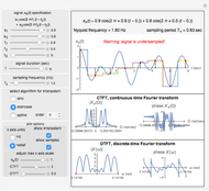
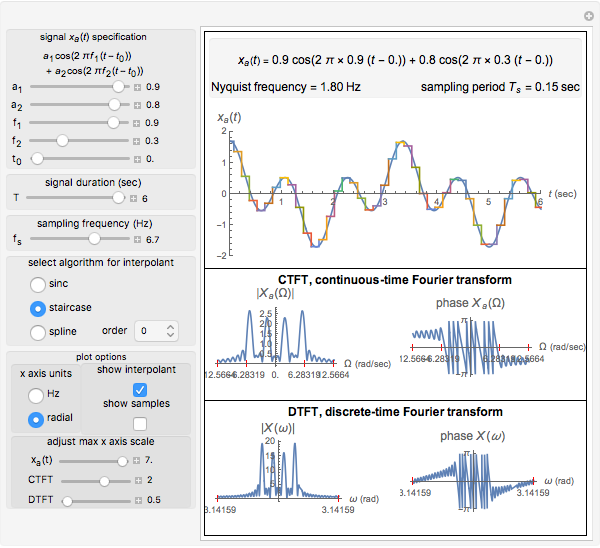
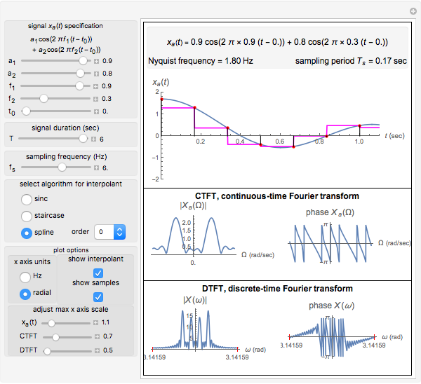
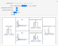
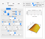
The purpose of this Demonstration is to show the relation between the continuous-time Fourier transform (CTFT) of a signal  and the corresponding discrete-time Fourier transform (DTFT) of the signal
  generated from
  ) by sampling.


Contributed by: Nasser M. Abbasi (March 2011)
Open content licensed under CC BY-NC-SA
Snapshots
Details
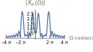
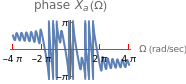
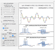
The CTFT of a continuous time signal is defined as 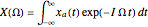 , where
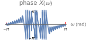
  is in radians per second. The DTFT of a discrete signal is defined as
 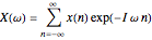 , where
  is in radians. In Mathematica, the built-in function FourierTransform implements the CTFT and the function FourierSequenceTransform implements the DTFT.
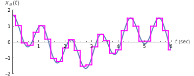
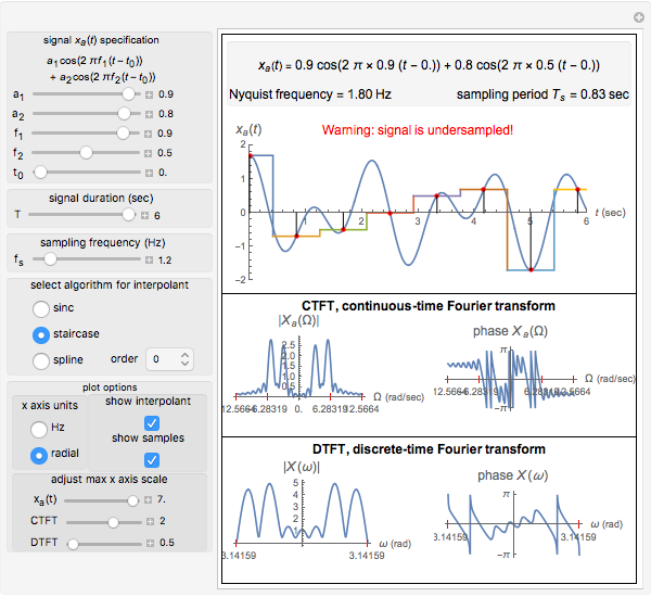
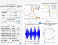
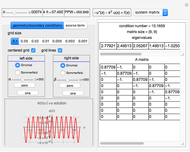
In this Demonstration, a signal made up of two harmonics is used to analyze the process of sampling and generating the DTFT. The signal is given by  , where
  is the frequency of each harmonic in cycles per second (Hz),
  is the amplitude of each harmonic in units appropriate to the nature of the signal (such as volts), and
  is the delay in seconds. The signal is of limited duration, which you can vary. Since is time-limited, its spectrum will not be band-limited. In practice, this is handled by passing the signal through an antialiasing filter before sampling it. This filter has not been implemented in this Demonstration, thus some aliasing will be present even if the sampling frequency is greater than the Nyquist frequency. For the purposes of this Demonstration, it was not necessary to implement an antialiasing filter before sampling.
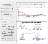
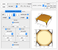
To reconstruct the time domain signal from the discrete time signal, one of the following algorithms can be selected: sinc interpolation, staircase interpolation, or spline interpolation (of order up to four). It was found that to obtain good reconstruction using the staircase and spline algorithms, the sampling frequency needs to be much higher than the Nyquist frequency.
You can vary the  axis plot range to see more details in the plot. Other plotting options are available to allow the change of units of the spectrum from Hz to radians and to superimpose the samples and the reconstructed signal on top of the original signal . This will show the effect of sampling.
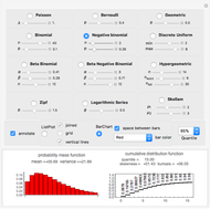
To reduce the signal to one harmonic only, you can set the amplitude of the other harmonic to zero. For a constant (DC) signal , you can set the frequencies of both harmonics to zero.
Permanent Citation
 Discrete Fourier Sine and Cosine Transforms
Daniel de Souza Carvalho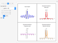 XFT: An Improved Fast Fourier Transform
Rafael G. Campos, J. Jesus Rico Melgoza, and Edgar Chavez XFT2D: A 2D Fast Fourier Transform
Rafael G. Campos, J. Jesus Rico Melgoza, and Edgar Chavez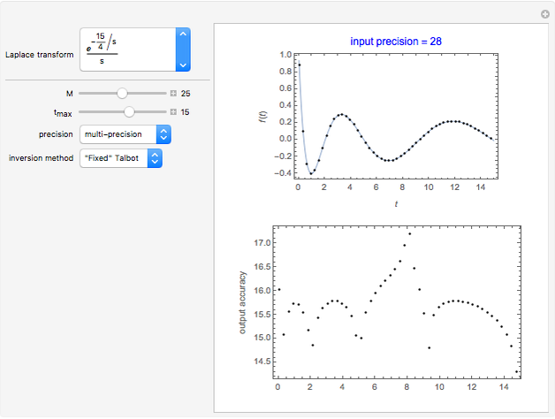 Comparing Four Methods of Numerical Inversion of Laplace Transforms (NILT)
Claude Montella and Jean-Paul Diard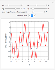 First and Second Derivatives of a Periodic Function Using Discrete Fourier Transforms
Housam Binous, Ahmed Bellagi, and Brian G. Higgins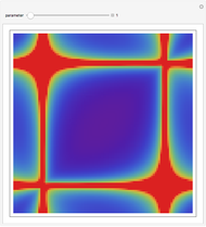 Fractional Fourier Transform
Enrique Zeleny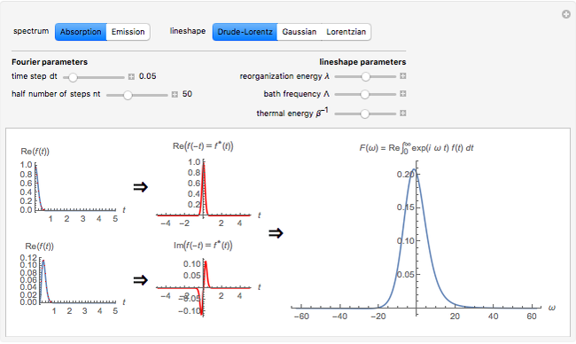 One-Sided Fourier Transform: Application to Linear Absorption and Emission Spectra
Liam Cleary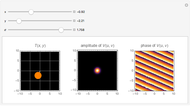 Amplitude and Phase in 2D Fourier Transforms
Katherine Rosenfeld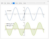 Synthesis with Even and Odd Functions
Aaron T. Becker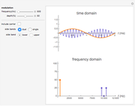 Amplitude Modulation
Jakub Serych
-
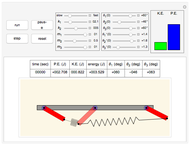
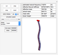
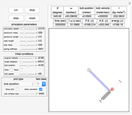
 Heavy Spring with Double Pendulum
Nasser M. Abbasi -
 Illustrating the Use of Discrete Distributions
Nasser M. Abbasi -
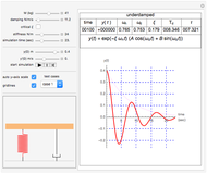
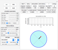
 Dynamic Analysis of a Second-Order System with Harmonic Loading
Nasser M. Abbasi -
 Cauchy and Engineering Strain Deformation in 3D
Nasser M. Abbasi -
 Dynamics of Two Cylinders with Three Springs
Nasser M. Abbasi -
 Principal Stresses and Mohr's Circle for Plane Stress
Nasser M. Abbasi -
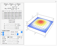
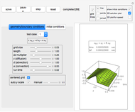
 Solving the 2D Poisson PDE by Eight Different Methods
Nasser M. Abbasi -
 Vibration of a Rectangular Membrane
Nasser M. Abbasi -
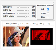 Selecting from ImageData Using Rows and Columns
Nasser M. Abbasi -
 Three Pendulums Connected by Two Springs
Nasser M. Abbasi -
 Wind Tower Structure Represented by Generalized Single Degree of Freedom
Nasser M. Abbasi -
 Free Response in a Second-Order System
Nasser M. Abbasi -
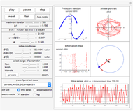 Chaotic Motion of a Damped Driven Pendulum: Bifurcation, Poincaré Map, Power Spectrum, and Phase Portrait
Nasser M. Abbasi -
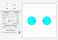 Particle Motion Simulation Using A Priori Collision Detection
Nasser M. Abbasi -
 Spring-Mass System on a Rotating Table
Nasser M. Abbasi -
 Solid Pendulum with a Spring-Mass System
Nasser M. Abbasi -
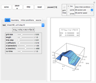
 Solving the Convection-Diffusion Equation in 1D Using Finite Differences
Nasser M. Abbasi -
 Solving the Diffusion-Advection-Reaction Equation in 1D Using Finite Differences
Nasser M. Abbasi -
 Solving the 1D Helmholtz Differential Equation Using Finite Differences
Nasser M. Abbasi -
 Solving the 2D Helmholtz Partial Differential Equation Using Finite Differences
Nasser M. Abbasi