Global B-Spline Surface Interpolation


Requires a Wolfram Notebook System
Interact on desktop, mobile and cloud with the free Wolfram Player or other Wolfram Language products.
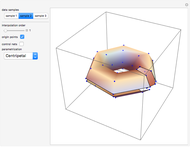
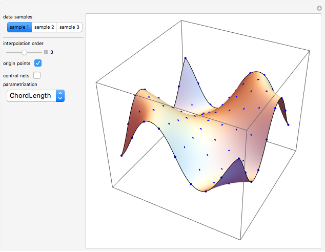
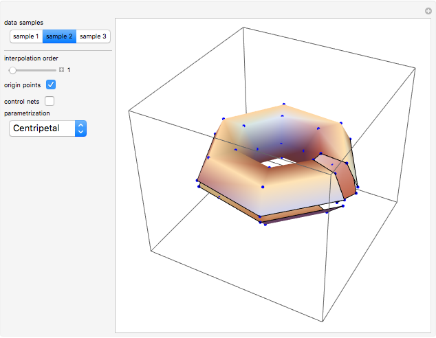
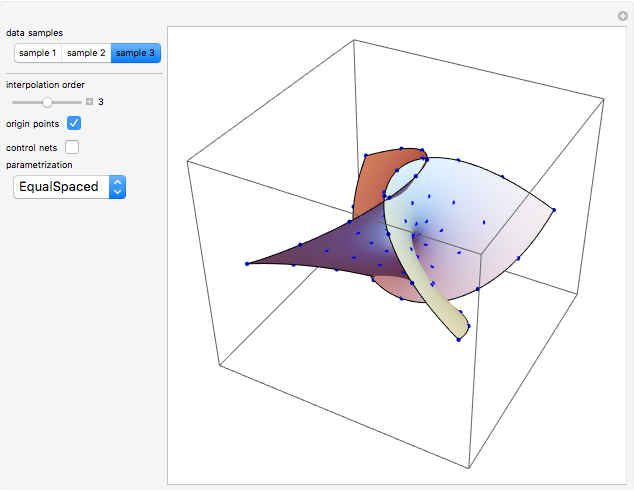
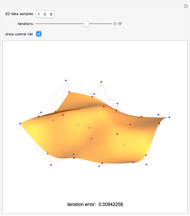
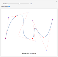
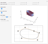
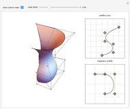
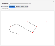
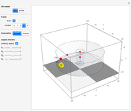
This Demonstration shows global B-spline surface interpolation. The implementation is fully described in the Details.
Contributed by: Shutao Tang (October 2015)
(Northwestern Polytechnical University, Xi'an City, China)
Open content licensed under CC BY-NC-SA
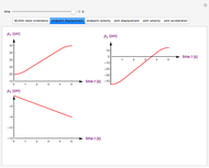
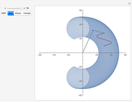
Snapshots


Details
Given a set of  data points
  ,
,  and
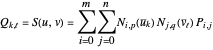
and  , this Demonstration constructs a nonrational
  -degree B-spline surface interpolating these points, namely:
 (1)
(1)
Again, the first order of business is to compute reasonable values for the  and the knot vectors
  and
and  . We show how to compute the
  ; the
; the  are analogous.
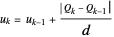
A common method is to use equations (2) or (3) to compute parameters  ,
,  , ⋯,
, ⋯,  for each
  and then to obtain each
  by averaging across all
  for
for  , that is,
 ,
,  ,
,
where for each fixed  ,
,  was computed by equation (2) or (3).
(a) Let  , then
 ,
,  for
for  , and
, and  . (2)
. (2)
(b) Let 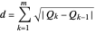 , then

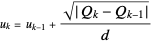 for
for  , and
, and  . (3)
. (3)
Once the  are computed, the knot vectors
  and
and  can be obtained by equation (4):
 ,
,  ,
,  ,
,  . (4)
. (4)
Now to the computation of the control points. Clearly, equation (1) represents  linear equations in the unknown
  . However, since
  is a tensor product surface, the
  can be obtained more simply and efficiently as a sequence of curve interpolations.
For fixed  , write equation (1) as
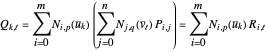 , (5)
, (5)
where 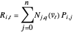 . (6)
. (6)
Notice that equation (5) is just curve interpolation through the points  . The
. The  are the control points of the isoparametric curve on
  at fixed
  . Now fixing
  and letting
  vary, equation (6) is curve interpolation through the points
  , with
  as the computed control points. Thus, the algorithm to obtain all the
  is as follows:
1. Using  and the
  , do
, do  curve interpolations through
  , which yields the
  .
.
2. Using  and the
  , do
, do  curve interpolations through
  , which yields the
  .
.
Reference
[1] L. Piegl and W. Tiller, The NURBS Book, 2nd ed., Berlin: Springer-Verlag, 1997 pp. 376–382.
Permanent Citation
 Algorithm for Bicubic Nonuniform B-Spline Surface Interpolation
Shutao Tang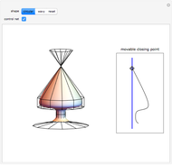 Shaping a Tubular B-Spline Surface
M. Szilvási-Nagy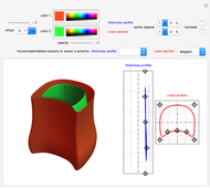 3D Object Designer Using Splines
Erik Mahieu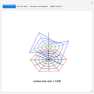 Series Approximation for the Schwarz D Surface
Brad Klee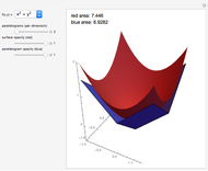 Finding the Area of a 3D Surface with Parallelograms
Mark Peterson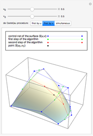 de Casteljau Algorithm for a Tensor-Product Bézier Surface
Isabelle Cattiaux-Huillard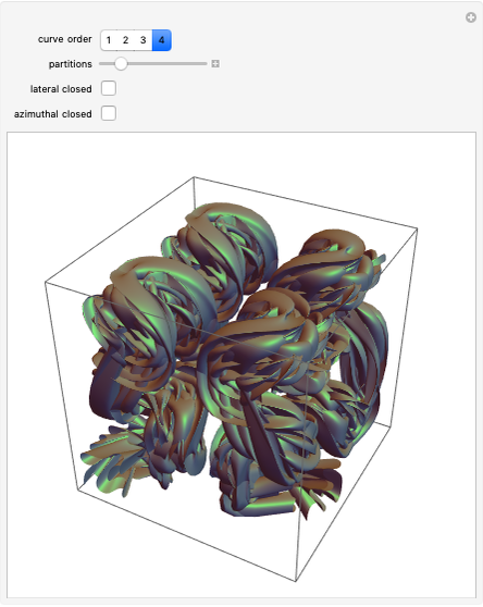 Interpolating the Hilbert Curve with a B-Spline to Create a Surface
Michael Trott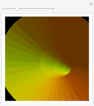 Traversing the Inside of a B-Spline Curve
Arnoud Buzing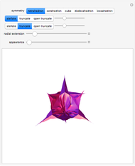 Platonic Spline Radiolari
Michael Trott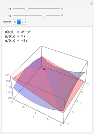 Tangent Planes to Quadratic Surfaces
Gerhard Schwaab and Chantal Lorbeer
-
 Algorithm for Cubic Nonuniform B-Spline Curve Interpolation
Shutao Tang -
Algorithm for Bicubic Nonuniform B-Spline Surface Interpolation
Shutao Tang -
 Cylindrical Surfaces from NURBS Curves
Shutao Tang -
 Constructing a Swung Surface around a B-Spline Curve
Shutao Tang -
 Global B-Spline Surface Interpolation
Shutao Tang -
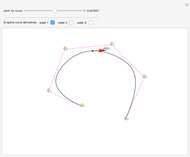
 Global B-Spline Curve Interpolation
Shutao Tang -
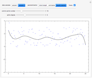 Global B-Spline Curve Fitting by Least Squares
Shutao Tang -
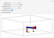 A Model of the SCARA Robot
Shutao Tang -
 The Derivative Vectors of a B-Spline
Shutao Tang -
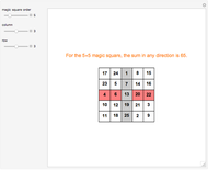 Magic Squares for Odd, Singly Even, and Doubly Even Orders
Shutao Tang -
 Generating a B-Spline Curve by the Cox-De Boor Algorithm
Shutao Tang -
 Calculating and Plotting B-Spline Basis Functions
Shutao Tang -
 Generating a Bezier Curve by the de Casteljau Algorithm
Shutao Tang -
 Forward and Inverse Kinematics of the SCARA Robot
Shutao Tang -
 Kinematics of SCARA Robot in 2D
Shutao Tang -
 A Two-Link Inverse-Kinematic Mechanism
Shutao Tang