Integrating across Singularities


Requires a Wolfram Notebook System
Interact on desktop, mobile and cloud with the free Wolfram Player or other Wolfram Language products.
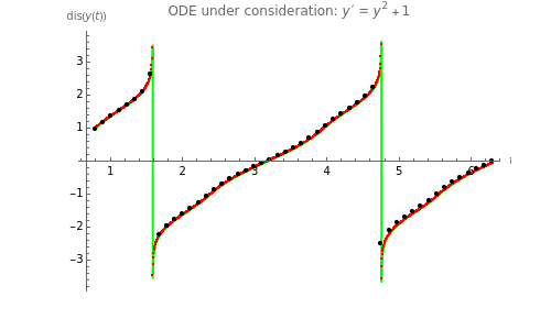
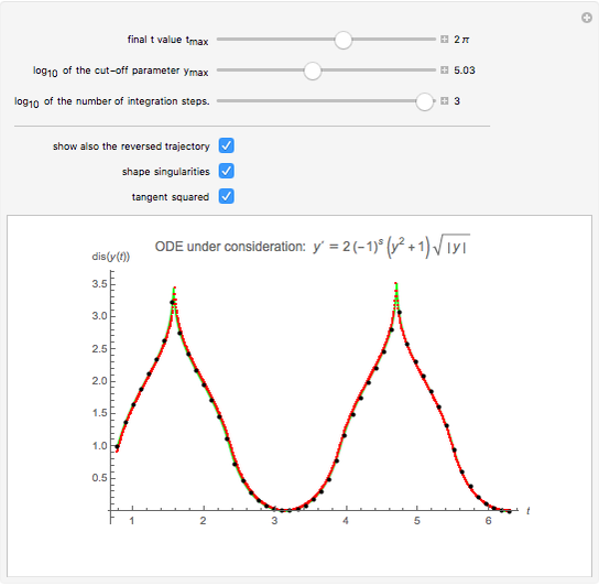
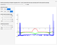
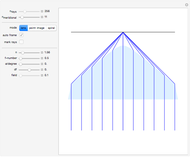
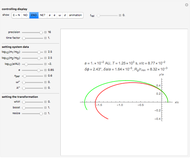
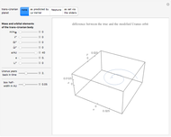
An initial value problem for a simple autonomous differential equation may develop singularities that prevent most time-discrete integrators from following the trajectory reliably. An example of this phenomenon is given by the ODE  , for which the initial condition
  yields the solution
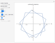
  . This ODE describes the rotation of a rigid body around an axis fixed in space in a formalism that describes the attitude of the body by Euler–Rodrigues parameters (instead of, say, Euler angles or orthogonal matrices). Thus we have a setting that asks for continuing the trajectory across the singularities, which occur whenever
  is
is  plus some integer multiple of
  .
.


Contributed by: Ulrich Mutze (March 2011)
Open content licensed under CC BY-NC-SA
Snapshots

Details
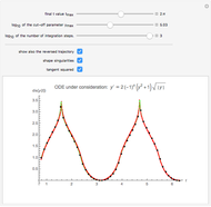
By checking the box "tangent squared", you replace the ODE by an ODE that is constructed such that its solution is  . For this
  we have
  . The sign factor has to switch whenever the trajectory passes a singularity and also when
  . As the program shows, the asynchronous leapfrog integrator can easily be made to do this switching. So it is not necessary to know in advance the values for which switching has to take place.
Snapshot 1:  adjusted for good representation of the exact solution
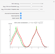
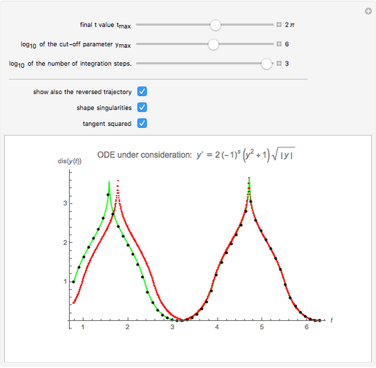
Snapshot 2: not so well adjusted; no good behavior of the reversed trajectory
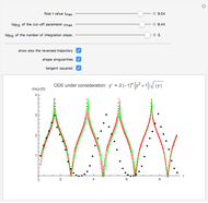
Snapshot 3: set too large; complete disorder after the first singularity
References
[1] Ulrich Mutze, An Asynchronous Leap-Frog Method, 2008. http://www.ma.utexas.edu/mp_arc/c/08/08-197.pdf.
[2] Alternate link for [1]: http://www.ulrichmutze.de/articles/leapfrog4.pdf.
[3] Ulrich Mutze, On Vectors, Points, Rotations, and Rigid Bodies. http://www.ulrichmutze.de/pedagogic_stuff/geo_10.pdf.
Permanent Citation
 Comparing Leapfrog Methods with Other Numerical Methods for Differential Equations
Ulrich Mutze Numerical Methods for Differential Equations
Edda Eich-Soellner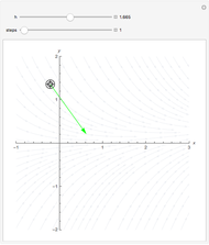 Understanding Runge-Kutta
Gerrard Liddell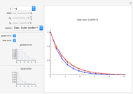 Global and Local Errors in Runge-Kutta Methods
Luis Rández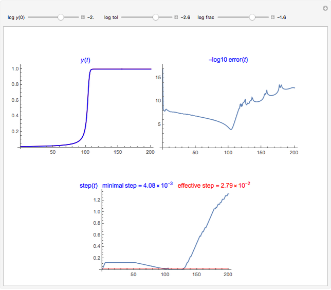 The Asynchronous Leapfrog Method as a Stiff ODE Solver
Ulrich Mutze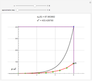 Euler's Method for the Exponential Function
Arnaud Crouzet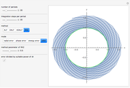 Testing Second-Order Integrators for Motion of a Charge in a Homogeneous Magnetic Field
Ulrich Mutze Numerical Integration Examples
Jason Beaulieu and Brian Vick Numerical Integration: Romberg's Method
Eugenio Bravo Sevilla Numerical Integration using Rectangles, the Trapezoidal Rule, or Simpson's Rule
Bartosz Naskrecki
-
 Simulating Real Gases in 2D
Ulrich Mutze -
Testing Second-Order Integrators for Motion of a Charge in a Homogeneous Magnetic Field
Ulrich Mutze -
 The Thomson Problem with Central Forces
Ulrich Mutze -
 Standard Colorimetric Observer Color-Matching Functions
Ulrich Mutze -
 Iteration Methods for Solving Kepler's Equation
Ulrich Mutze -
 Approach of a System of Particles towards Thermal Equilibrium
Ulrich Mutze -
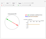 Monte Carlo Simulation of Two-Electron Spin Correlations
Ulrich Mutze -
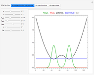 Eigenfunctions of a 1D Quantum System with Adjustable Potential
Ulrich Mutze -
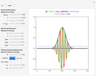 Quantum Dynamics in 1D
Ulrich Mutze -
 Lens Aberrations
Ulrich Mutze -
 On the Stability Limit of Leapfrog Methods
Ulrich Mutze -
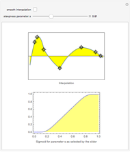 Smoothly Interpolating a Set of Data
Ulrich Mutze -
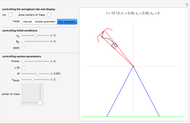 Swingboat Ride
Ulrich Mutze -
 The Gravitational Two-Body Problem in the Einstein-Infeld-Hoffmann Approximation
Ulrich Mutze -
 Contracting the Double-Twist in SO(3)
Ulrich Mutze -
The Asynchronous Leapfrog Method as a Stiff ODE Solver
Ulrich Mutze -
 Model for Crystallization in 2D
Ulrich Mutze -
 Time Evolution of a Symmetric System
Ulrich Mutze -
 Relativistic Quantum Dynamics in 1D and the Klein Paradox
Ulrich Mutze -
 The Uranus Puzzle
Ulrich Mutze