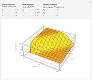
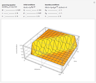
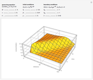
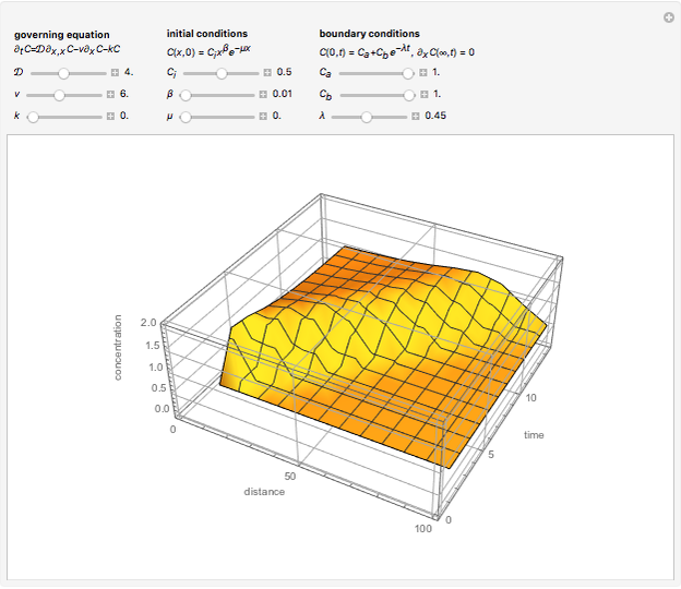
Mixing Cell Model Applied to Transport in Porous Media
Initializing live version


Requires a Wolfram Notebook System
Interact on desktop, mobile and cloud with the free Wolfram Player or other Wolfram Language products.
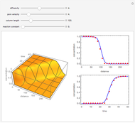
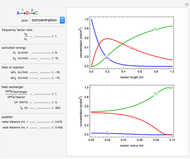
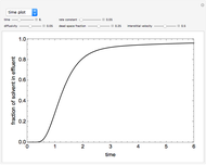
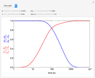
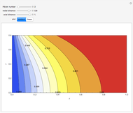
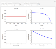
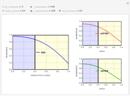
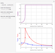
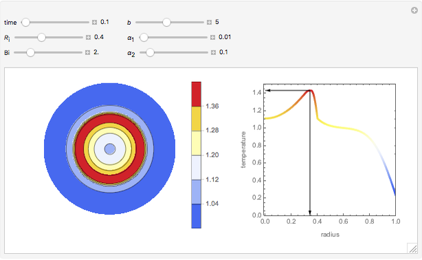
The mixing cell model is used to solve the diffusion-advection equation with complex initial and boundary conditions.
[more]


Contributed by: Clay Gruesbeck (October 2015)
Open content licensed under CC BY-NC-SA
Snapshots


Details
Reference
[1] H. C. Van Ommen, "The 'Mixing-Cell' Concept Applied to Transport of Non-reactive and Reactive Components in Soils and Groundwater," Journal of Hydrology, 78(3–4), 1985 pp. 201–213. doi:10.1016/0022-1694(85)90101-5.
Permanent Citation
Related Demonstrations
More by Author
 Mixing-Cell Model for the Diffusion-Advection Equation
Clay Gruesbeck Absorption in a Falling Thin Liquid Film at Low Reynolds Numbers
Housam Binous and Brian G. Higgins The Pigford Problem
Jorge Gamaliel Frade Chávez Numerical Solution of Some Fractional Diffusion Equations
Santos Bravo Yuste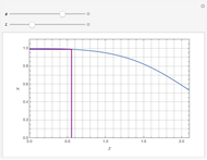 Unsteady-State Evaporation in an Infinite Tube
Jorge Gamaliel Frade Chávez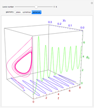 Nonstationary Heat and Mass Transfer in a Porous Catalyst Particle
Housam Binous, Abdullah A. Shaikh, and Ahmed Bellagi Mixing in Two Connected Tanks
Stephen Wilkerson Thermal Diffusivity of a Sphere
Clay Gruesbeck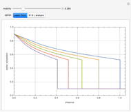 Two-Phase Fluid Flow in Porous Media
Clay Gruesbeck Potential Flow over an Airfoil Specified by Numerical Data File
Richard L. Fearn
-
 Radial and Axial Variations in a Nonisothermal Tubular Reactor
Clay Gruesbeck -
 Miscible Displacement of Oil in Heterogenous Porous Media
Clay Gruesbeck -
 Simultaneous Heat and Moisture Transfer in a Porous Cylinder
Clay Gruesbeck -
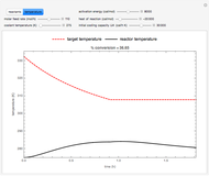 Safe Operation of a Semibatch Reactor
Clay Gruesbeck -
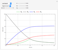 Parallel Nonisothermal Reactions in Batch and Semibatch Reactors
Clay Gruesbeck -
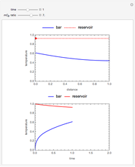 Heat Transfer between a Bar and a Fluid Reservoir: A Coupled PDE-ODE Model
Clay Gruesbeck -
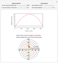 External Ballistics of Rifle Bullets
Clay Gruesbeck -
 Extended Graetz Problem
Clay Gruesbeck -
 Heat Transport and Chemical Reaction in Tubular Reactor with Laminar Flow
Clay Gruesbeck -
 Transient Cooling of Composite Solids
Clay Gruesbeck -
 Concurrent and Countercurrent Cooling in Tubular Reactors with Exothermic Chemical Reactions
Clay Gruesbeck -
 Transient Heat Conduction with a Nuclear Heat Source
Clay Gruesbeck -
 Controlled Release of a Drug from a Hemispherical Matrix
Clay Gruesbeck -
 Cooling of a Composite Slab
Clay Gruesbeck -
 Unsteady-State Heat Conduction in a Cylinder
Clay Gruesbeck -
 Adsorption, Diffusion and Chemical Reaction in a Slab
Clay Gruesbeck -
 Diffusion and Reaction in a Falling Liquid Film
Clay Gruesbeck -
 Freezing of Water around a Heat Sink
Clay Gruesbeck -
Thermal Diffusivity of a Sphere
Clay Gruesbeck -
 Transport and Deposition of Colloid in Rock Fractures
Clay Gruesbeck