Rectangular Pulse and Its Fourier Transform

Requires a Wolfram Notebook System
Interact on desktop, mobile and cloud with the free Wolfram Player or other Wolfram Language products.
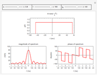
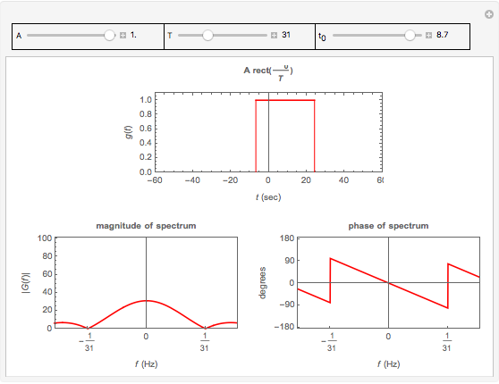
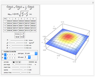
This Demonstration illustrates the relationship between a rectangular pulse signal and its Fourier transform. There are three parameters that define a rectangular pulse: its height  , width
  in seconds, and center
  . Mathematically, a rectangular pulse delayed by
  seconds is defined as
  and its Fourier transform or spectrum is defined as
  .
.

Contributed by: Nasser M. Abbasi (March 2011)
Open content licensed under CC BY-NC-SA
Snapshots


Details
This Demonstration illustrates the following relationship between a rectangular pulse and its spectrum:
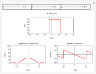
1. As the pulse becomes flatter (i.e., the width  of the pulse increases), the magnitude spectrum loops become thinner and taller. In other words, the zeros (the crossings of the magnitude spectrum with the
  axis) move closer to the origin. In the limit, as
  becomes very large, the magnitude spectrum approaches a Dirac delta function located at the origin.
2. As the height of the pulse become larger and its width becomes smaller, it approaches a Dirac delta function and the magnitude spectrum flattens out and becomes a constant of magnitude 1 in the limit.
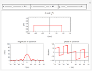
3. As  changes, the pulse shifts in time, the magnitude spectrum does not change, but the phase spectrum does.
4. We notice a  phase shift at each frequency defined by
  , where
  is an integer other than zero, and
  is the pulse duration. These frequencies are the zeros of the magnitude spectrum.
Permanent Citation
 XFT: An Improved Fast Fourier Transform
Rafael G. Campos, J. Jesus Rico Melgoza, and Edgar Chavez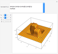 XFT2D: A 2D Fast Fourier Transform
Rafael G. Campos, J. Jesus Rico Melgoza, and Edgar Chavez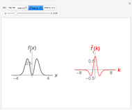 Fourier Transform Pairs
Porscha McRobbie and Eitan Geva Distance Transforms
Henry Kwong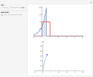 Convolution with a Rectangular Pulse
Carsten Roppel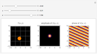 Amplitude and Phase in 2D Fourier Transforms
Katherine Rosenfeld Fractional Fourier Transform
Enrique Zeleny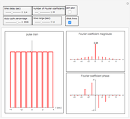 Fourier Series Coefficients of a Rectangular Pulse Signal
Nasser M. Abbasi Numerical Inversion of the Laplace Transform: The Fourier Series Approximation
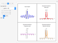
Housam Binous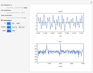 Discrete Fourier Transform of a Two-Tone Signal
Carsten Roppel
-
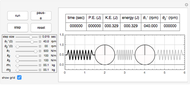
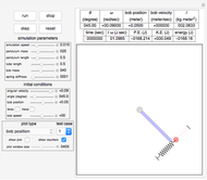
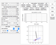 Heavy Spring with Double Pendulum
Nasser M. Abbasi -
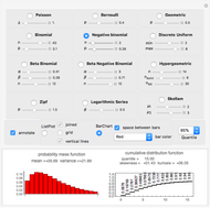 Illustrating the Use of Discrete Distributions
Nasser M. Abbasi -
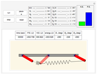
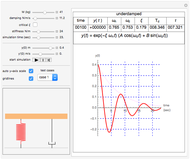
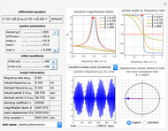 Dynamic Analysis of a Second-Order System with Harmonic Loading
Nasser M. Abbasi -
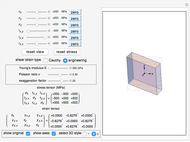 Cauchy and Engineering Strain Deformation in 3D
Nasser M. Abbasi -
 Dynamics of Two Cylinders with Three Springs
Nasser M. Abbasi -
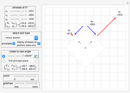 Principal Stresses and Mohr's Circle for Plane Stress
Nasser M. Abbasi -
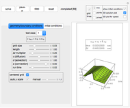
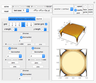
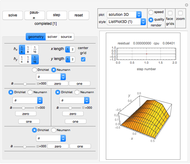 Solving the 2D Poisson PDE by Eight Different Methods
Nasser M. Abbasi -
 Vibration of a Rectangular Membrane
Nasser M. Abbasi -
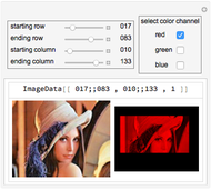 Selecting from ImageData Using Rows and Columns
Nasser M. Abbasi -
 Three Pendulums Connected by Two Springs
Nasser M. Abbasi -
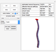 Wind Tower Structure Represented by Generalized Single Degree of Freedom
Nasser M. Abbasi -
 Free Response in a Second-Order System
Nasser M. Abbasi -
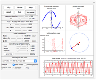 Chaotic Motion of a Damped Driven Pendulum: Bifurcation, Poincaré Map, Power Spectrum, and Phase Portrait
Nasser M. Abbasi -
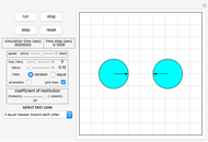 Particle Motion Simulation Using A Priori Collision Detection
Nasser M. Abbasi -
 Spring-Mass System on a Rotating Table
Nasser M. Abbasi -
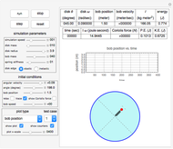
 Solid Pendulum with a Spring-Mass System
Nasser M. Abbasi -
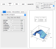
 Solving the Convection-Diffusion Equation in 1D Using Finite Differences
Nasser M. Abbasi -
 Solving the Diffusion-Advection-Reaction Equation in 1D Using Finite Differences
Nasser M. Abbasi -
 Solving the 1D Helmholtz Differential Equation Using Finite Differences
Nasser M. Abbasi -
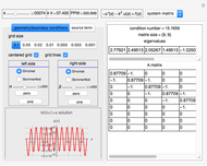
 Solving the 2D Helmholtz Partial Differential Equation Using Finite Differences
Nasser M. Abbasi