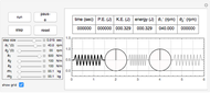
Spinning Disk Pendulum Swinging on Top of a Rotating Table


Requires a Wolfram Notebook System
Interact on desktop, mobile and cloud with the free Wolfram Player or other Wolfram Language products.
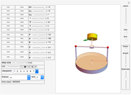
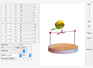
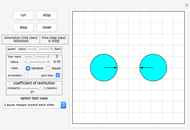
This Demonstration shows a pendulum with a small spinning rigid cylindrical bob in which the pendulum rod (assumed to have negligible mass) swings from a frame fixed on top of a rotating table. The system has three degrees of freedom: the pendulum swing angle  , the spin angle
  of the pendulum bob, and the rotation angle
  of the large table.
Contributed by: Nasser M. Abbasi (July 2011)
Open content licensed under CC BY-NC-SA
Snapshots


Details
The kinetic energy of the system is given by

and the potential energy by  , where
  is the moment of inertia of the large table,
  is its mass, and
  is its radius.
  ,
,  , and
, and  are the moments of inertia of the bob around its principal axis; due to symmetry,
 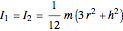 and
and  , where
  is the radius of the bob,
  is the height of the bob cylinder, and
  is its mass. Using the parallel axis theorem, the moment of inertia tensor
  for the bob is found relative to the point where the pendulum rod is attached to the frame. The angular momentum vector
  is found relative to this point and not relative to the center of mass of the bob.
The absolute rate of change of the angular momentum vector  is found using
  , where
  is the rate of change of relative to the fixed point described above. All the terms above are vectors and the product
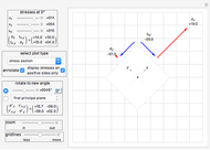
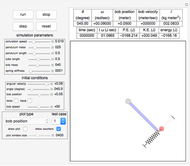
  is the vector cross product. You can see these vectors and their components visually displayed by selecting a display option from the popup menu. A special case occurs when the bob is spinning around one of its principal axes. In this case you will see that the and vectors are always parallel.
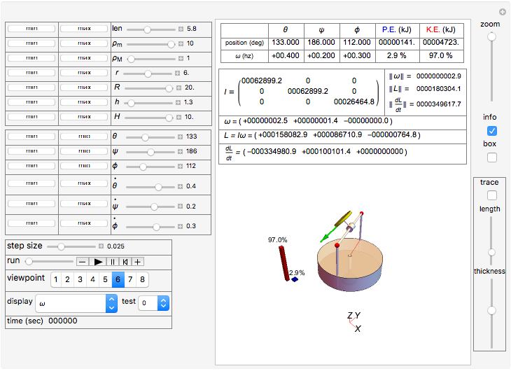
The following is a description of the items on the top half of the left panel of the controls:  is the length of the pendulum rod,
  is the density of the material of the bob cylinder,
  is the density of the material of the large table cylinder, is the radius of the bob cylinder, is the radius of the large table cylinder, is the height of the bob cylinder, and
  is the height of the large table cylinder.
The panel below that contains the initial conditions for the three rotation angles , , and . The units for the angles are in degrees with the range 0–360°. The units for the angular velocities are in hz in the range of  to
to  . For convenience, small buttons are placed next to the sliders to set the initial condition to its minimum or maximum value.
The slider labeled "step size" can be used to adjust the animation rate. The smaller the step size, the more accurate the simulation will be, but the longer and slower it will run.
The popup menu labeled "display" lets you select which vectors to view while the simulation is running. You can select the angular momentum or the rate of the angular momentum  of the bob. Or select to view the angular velocity vector of the center of gravity of the bob, which is given by
 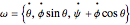 .
.
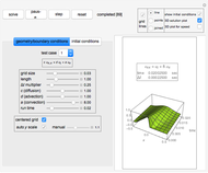
A number of test cases is available to try. When you select one of these, the control variables are automatically set to preset values. Then you can click the run button to see the selected test case using those values. When running a specific case, you will not be able adjust any of the controls other than changing to a different case. Selecting the special test case 0 releases that, allowing you to adjust other control variables.
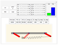
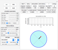
If you click the "info" checkbox on the right side of the display, the following information is displayed when running: the moment of inertia tensor , the angular momentum vector , the rate of change of the angular momentum vector , and the current values of the three angles , , and and their angular velocities. The current value of the system kinetic energy (K.E.) and potential energy (P.E.) are given in kilojoules (KJ).
The current time in seconds is shown at the lower side of the left part of the display. A "zoom" slider can be used to zoom into the display while it is running. This provides limited zooming capability. You can use the built-in Mathematica support for zoom and panning by clicking the display then using the Ctrl key. See Mathematica documentation for more information. If you decide to use the built-in zooming instead of the "zoom" slider, you should pause the simulation first to obtain better control of the zooming action, then you can resume the simulation.
The "trace" checkbox on the right side lets you trace the trajectory of the center of mass of the bob as it moves in 3D inertial space. You can adjust the length of the trace trajectory using the "length" slider below the "trace" checkbox and the thickness of the trace line using the "thickness" slider. The trace can be cleared at anytime by clicking the "trace" checkbox again.
When the rate of the angular momentum of the bob is not zero, there must exist a torque  to account for this, which is given by
  . The torque is not displayed in this version of the Demonstration. It is generated by support reaction from the ground.
References
[1] D. T. Greenwood, Principles of Dynamics, Upper Saddle River, NJ: Prentice Hall, 1965, Chapter 8.
[2] R. P. Feynman, R. B. Leighton, and M. L. Sands, The Feynman Lectures on Physics, Reading, MA: Addison–Wesley, 1963, pp. 20–1 to 20–8.
Permanent Citation
 Rigid Body Pendulum on a Flywheel
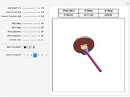
Nasser M. Abbasi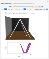 Pendulum Waves
Stan Wagon (Macalester College) and S. M. Blinder Stationary Precession of a Spinning Top
William C. Guttner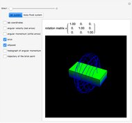 Free Rotation of an Asymmetric Top
Ferat Talat oglu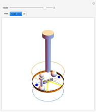 Torsion Pendulum
Enrique Zeleny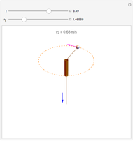 Spinning Mass with Variable Radius
Enrique Zeleny Conic Pendulum
Enrique Zeleny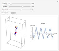 Vibrating Inverted Pendulum
Kay Herbert Bead on a Rotating Wire
Ryan K. Smith (Wolfram Research) Impulse Acting on a Pendulum
Sarah Lichtblau
-
 Heavy Spring with Double Pendulum
Nasser M. Abbasi -
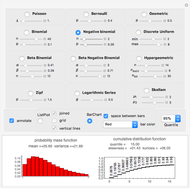 Illustrating the Use of Discrete Distributions
Nasser M. Abbasi -
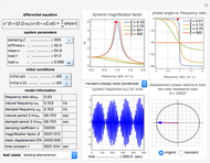 Dynamic Analysis of a Second-Order System with Harmonic Loading
Nasser M. Abbasi -
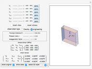 Cauchy and Engineering Strain Deformation in 3D
Nasser M. Abbasi -
 Dynamics of Two Cylinders with Three Springs
Nasser M. Abbasi -
 Principal Stresses and Mohr's Circle for Plane Stress
Nasser M. Abbasi -
 Solving the 2D Poisson PDE by Eight Different Methods
Nasser M. Abbasi -
 Vibration of a Rectangular Membrane
Nasser M. Abbasi -
 Selecting from ImageData Using Rows and Columns
Nasser M. Abbasi -
 Three Pendulums Connected by Two Springs
Nasser M. Abbasi -
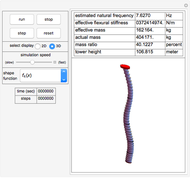 Wind Tower Structure Represented by Generalized Single Degree of Freedom
Nasser M. Abbasi -
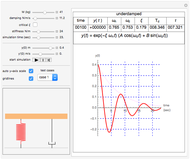 Free Response in a Second-Order System
Nasser M. Abbasi -
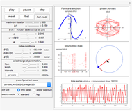 Chaotic Motion of a Damped Driven Pendulum: Bifurcation, Poincaré Map, Power Spectrum, and Phase Portrait
Nasser M. Abbasi -
 Particle Motion Simulation Using A Priori Collision Detection
Nasser M. Abbasi -
 Spring-Mass System on a Rotating Table
Nasser M. Abbasi -
 Solid Pendulum with a Spring-Mass System
Nasser M. Abbasi -
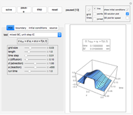
 Solving the Convection-Diffusion Equation in 1D Using Finite Differences
Nasser M. Abbasi -
 Solving the Diffusion-Advection-Reaction Equation in 1D Using Finite Differences
Nasser M. Abbasi -
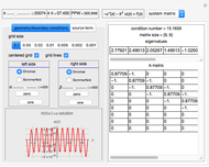 Solving the 1D Helmholtz Differential Equation Using Finite Differences
Nasser M. Abbasi -
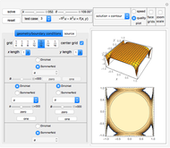 Solving the 2D Helmholtz Partial Differential Equation Using Finite Differences
Nasser M. Abbasi