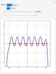
Hopf Bifurcations in a Nonlinear Two-Dimensional Autonomous System
Initializing live version


Requires a Wolfram Notebook System
Interact on desktop, mobile and cloud with the free Wolfram Player or other Wolfram Language products.
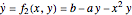
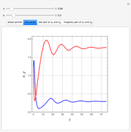
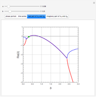
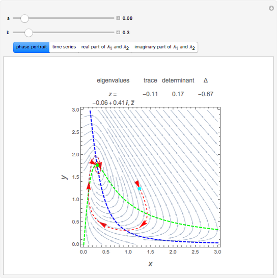
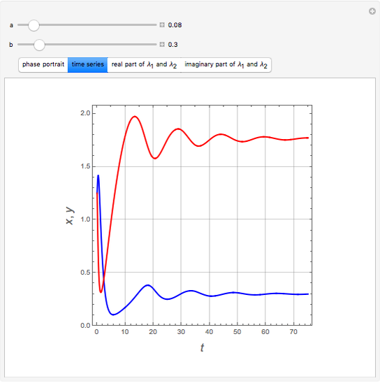
In the study of nonlinear dynamics, it is useful to first introduce students to simple systems that exhibit periodic behavior as a consequence of a Hopf bifurcation. The two-dimensional nonlinear and autonomous system given by
[more]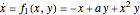


Contributed by: Housam Binous, Ahmed Bellagi, and Brian G. Higgins (October 2013)
Open content licensed under CC BY-NC-SA
Snapshots

Details
Reference
[1] P. Gray and S. K. Scott, Chemical Oscillations and Instabilities: Non-Linear Chemical Kinetics, Oxford: Clarendon Press, 1994.
Permanent Citation
Related Demonstrations
More by Author
 Asymptotic Stability of Dynamical System by Lyapunov's Direct Method
Housam Binous and Ahmed Bellagi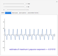 Study of the Dynamic Behavior of the Lorenz System
Housam Binous and Zakia Nasri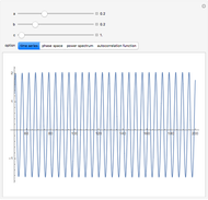 Study of the Dynamic Behavior of the Rossler System
Housam Binous and Zakia Nasri KAM Tori Reforming
Marco Frasca Particle Moving around Two Extreme Black Holes
Enrique Zeleny V.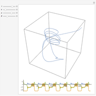 Gavrilov-Shilnikov Model
Enrique Zeleny Moore-Spiegel Attractor
Milena Cuellar Pen Falling Off a Finger
Michael Trott Double Pendulum
Rob Morris Phase Space of an Intermittently Driven Oscillator
Manu P. John and V. M. Nandakumaran
-
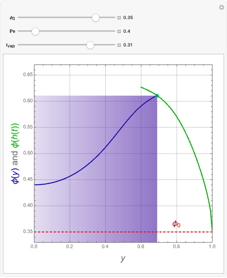 Distribution of Colloidal Particles during Solvent Evaporation
Brian G. Higgins -
 Heat Conduction in a Rod
Brian G. Higgins -
 A Graphically Enhanced Method for Computing Real Roots of Nonlinear Functions
Brian G. Higgins -
 All Real Roots of a Nonlinear System of Equations
Brian G. Higgins -
 Seader's Method for Real Roots of a Nonlinear Equation
Brian G. Higgins -
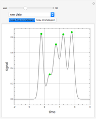 Analysis of Chromatographic Data
Brian G. Higgins -
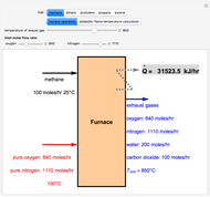 Combustion Reactions in a Furnace
Brian G. Higgins -
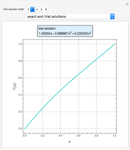 Boundary Value Problem Using Galerkin's Method
Brian G. Higgins -
 Operation of an Ethane Steam Cracker
Brian G. Higgins -
 Gibbs Free Energy Minimization Applied to the Haber Process
Brian G. Higgins -
 Minimum of a Function Using the Fibonacci Sequence
Brian G. Higgins -
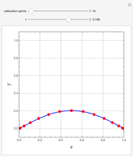
 Transient Heat Conduction Using Chebyshev Collocation
Brian G. Higgins -
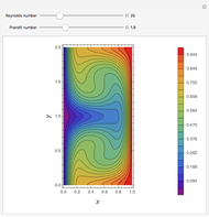 Steady-State Two-Dimensional Convection-Diffusion Equation
Brian G. Higgins -
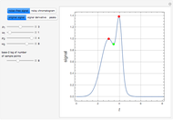 Peak Retention Time Using Discrete Fourier Transform
Brian G. Higgins -
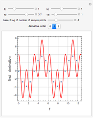 First and Second Derivatives of a Periodic Function Using Discrete Fourier Transforms
Brian G. Higgins -
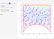 Stokes Flow in Container with Concave Bottom
Brian G. Higgins -
 Cooling with a Shaped Pin Fin
Brian G. Higgins -
 Solution of the Laplace Equation Using Coordinates Fitted to the Boundary Conditions
Brian G. Higgins -
 Flow Through a Rectangular Duct
Brian G. Higgins -
 Flow through Chamfered Ducts
Brian G. Higgins