Adaptive Monte Carlo Integration


Requires a Wolfram Notebook System
Interact on desktop, mobile and cloud with the free Wolfram Player or other Wolfram Language products.
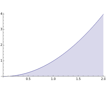
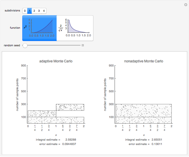
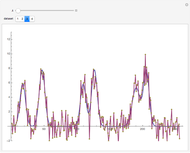
This Demonstration compares adaptive and nonadaptive Monte Carlo integration for two different functions,  and
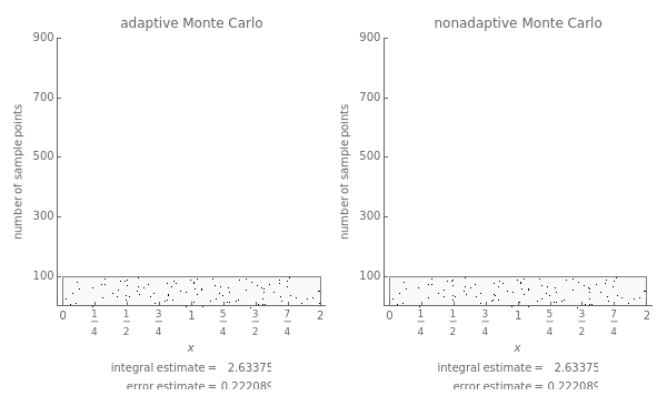
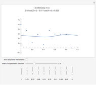
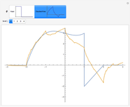
and  . The plot shows the places on the interval
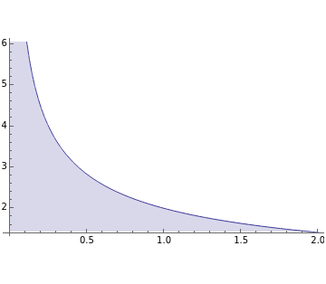
  where sample points are added as the number of sample points is increased. The actual values of the integrals to six significant figures are 2.66667 and 5.65685. The adaptive technique generally gets better estimates with the same number of sample points by subdividing the subinterval with the highest error estimate. Normally this process would be repeated until some error criterion is satisfied, but in this Demonstration only four subdivisions are shown.
Contributed by: Sijia Liang and Bruce Atwood (January 2013)
(Beloit College)
Open content licensed under CC BY-NC-SA
Snapshots


Details
In one dimension, if  is integrable on the interval
  , then the average value of is
  . From this, the nonadaptive (basic) Monte Carlo method estimates the integral by
  , where
  is the mean of the function evaluated at
  randomly sampled points. The corresponding error estimate is
  , where
  is the variance of the function evaluations. Thus the error can be reduced by increasing the number of sample points or reducing the variance. The key idea of adaptive Monte Carlo is to reduce the variance by recursive subdivision. Parts of this Demonstration are modifications of examples from the Wolfram Mathematica Documentation Center tutorial "Advanced Numerical Integration in Mathematica" (see link below). Students should try to explain why Monte Carlo integration has more difficulty for the function with the singularity at 0. (Hint: look at the formulas for the integral estimate and error estimate.)
Permanent Citation
 Monte Carlo Estimation of Area
Mark D. Normand and Micha Peleg Area Bisectors via Monte Carlo
Ed Pegg Jr Approximating Pi by the Monte Carlo Method
Zubeyir Cinkir Numerical Integration using Rectangles, the Trapezoidal Rule, or Simpson's Rule
Bartosz Naskrecki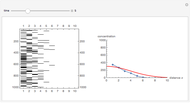 Simulation of 1D Diffusion Using the Monte Carlo Method
Quang-Dao Trinh Monte Carlo Methods to Estimate Area
Tomas Garza Two-Dimensional Integrals Using the Monte Carlo Method
Housam Binous, Brian G. Higgins, and Ahmed Bellagi Integration by Riemann Sums
Jiwon Hwang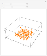 Simulation of 3D Diffusion Using the Monte Carlo Method
Quang-Dao Trinh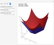 Finding the Area of a 3D Surface with Parallelograms
Mark Peterson
-
 Trigonometric Fitting and Interpolation
Bruce Atwood -
 Balancing a Can on Its Edge
Bruce Atwood -
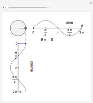 Spinning Out Sine and Cosine
Bruce Atwood -
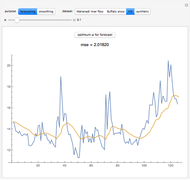 Forecasting with Exponential Moving Averages
Bruce Atwood -
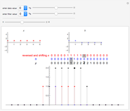 Convolution Sum
Bruce Atwood -
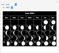 Lunar Calendar Maker
Bruce Atwood -
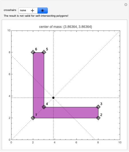 Center of Mass of a Polygon
Bruce Atwood -
 Projection into Spaces Generated by Haar and Daubechies Scaling Functions
Bruce Atwood -
 Adaptive Monte Carlo Integration
Bruce Atwood -
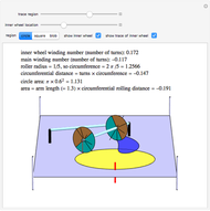 The Polar Planimeter
Bruce Atwood -
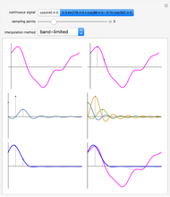 Reconstructing a Sampled Signal Using Interpolation
Bruce Atwood -
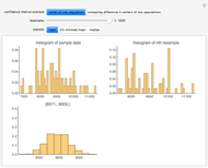 Bootstrap Percentile Confidence Intervals
Bruce Atwood -
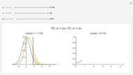 Power Curve of a Mean Test
Bruce Atwood -
 Approximating Continuous Functions with Haar Approximations
Bruce Atwood -
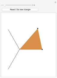 Sliding to the Fermat Point
Bruce Atwood -
 Wavelet Shrinkage Denoising
Bruce Atwood -
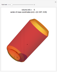
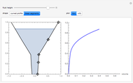 Filling a Container Defined by a Curve
Bruce Atwood -
 Squeeze Theorem
Bruce Atwood -
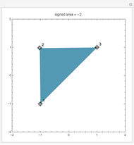 Signed Area of a Polygon
Bruce Atwood -
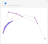 Bézier Curve by de Casteljau's Algorithm
Bruce Atwood