Integrating "Beyond Infinity" and Back


Requires a Wolfram Notebook System
Interact on desktop, mobile and cloud with the free Wolfram Player or other Wolfram Language products.
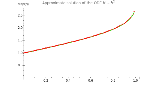
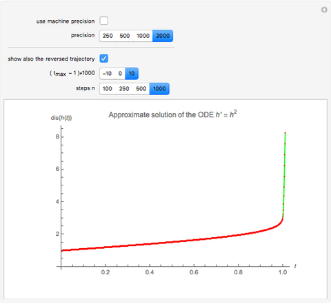
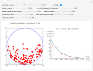
Consider the simple ordinary differential equation  with initial condition
  . The solution is obviously given by
  . It tends to infinity as
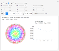
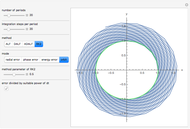
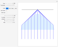
  tends to 1. We now consider a time-discrete approximation to this solution as provided by the asynchronous leapfrog method. Since the evolution step formula does not involve potentially undefined operations, any such discrete approximation is well defined for all its values. Of course, the approximated
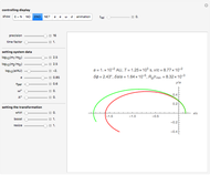
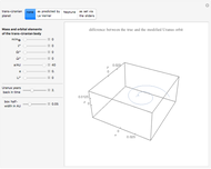
  values grow dramatically and will soon transcend what can be represented even with Mathematica's arbitrary-precision numbers. Since the asynchronous leapfrog method is a reversible integration method, we should be able to go along each finite discrete trajectory back to its initial point. If the final point was "close to infinity", the computation needs to be done with a large number of digits in order to come back to its initial point. This is what the present Demonstration studies. Values are input by means of setter bars instead of sliders since updating the curve for higher precision and
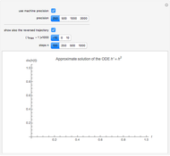
  may take a few seconds. (This does not affect Autorun, which uses machine precision throughout.) The reversed trajectory is marked by red dots and one easily sees (if the box 'show also the reversed trajectory' is activated) whether the reversed trajectory reaches the initial point. In all cases where it fails to do so, increasing the value of precision will finally solve the problem. In some cases, precision up to 2000 is needed.

Contributed by: Ulrich Mutze (March 2011)
Open content licensed under CC BY-NC-SA
Snapshots


Details
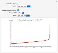
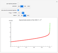
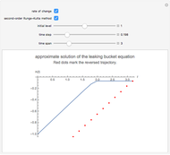
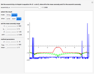
Snapshot 1: Maximum stress, reaching the largest numbers. The integration is from  to
to  with
with  ; precision 1000 turns out to be insufficient for reversibility.
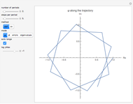
Snapshot 2: Reversible trajectory that gets lost in machine precision. Here the integration is from to with  ; due to the larger value of
  , there are fewer steps in the critical domain
  and the values are less gigantic; so a precision of 250 is sufficient for getting a reversible trajectory.
Snapshot 3: Using machine precision, together with the remaining settings of Snapshot 2, spoils reversibility.
References
[1] Ulrich Mutze An Asynchronous Leap-Frog Method, 2008., http://www.ma.utexas.edu/mp_arc/c/08/08-197.pdf.
[2] Alternate link for [1]: http://www.ulrichmutze.de/articles/leapfrog4.pdf.
Permanent Citation
 Leaking Bucket Equation and Reversibility
Ulrich Mutze Trigonometric Integral Functions
Rob Morris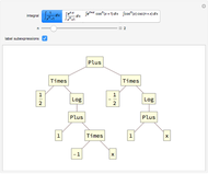 Expression Trees for Integrals
Stephen Wolfram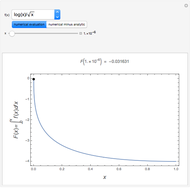 Numerical Evaluation of Some Definite Integrals
Mikhail Dimitrov Mikhailov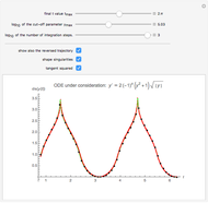 Integrating across Singularities
Ulrich Mutze Integrating Some Rational Functions
Izidor Hafner The Geometry of Integrating a Power around the Origin
John Custy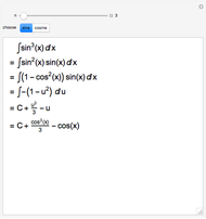 Integrating Odd Powers of Sine and Cosine by Substitution
George Beck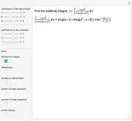 Integrating a Rational Function with a Cubic Denominator with One Real Root
Izidor Hafner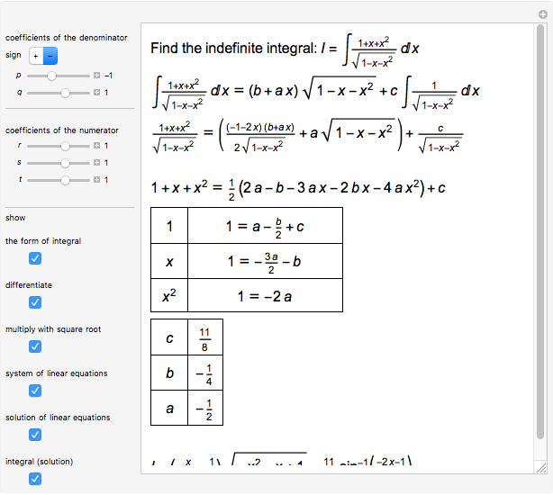 Integrating a Quadratic Divided by the Square Root of a Quadratic
Izidor Hafner
-
 Simulating Real Gases in 2D
Ulrich Mutze -
 Testing Second-Order Integrators for Motion of a Charge in a Homogeneous Magnetic Field
Ulrich Mutze -
 The Thomson Problem with Central Forces
Ulrich Mutze -
 Standard Colorimetric Observer Color-Matching Functions
Ulrich Mutze -
 Iteration Methods for Solving Kepler's Equation
Ulrich Mutze -
 Approach of a System of Particles towards Thermal Equilibrium
Ulrich Mutze -
 Monte Carlo Simulation of Two-Electron Spin Correlations
Ulrich Mutze -
 Eigenfunctions of a 1D Quantum System with Adjustable Potential
Ulrich Mutze -
 Quantum Dynamics in 1D
Ulrich Mutze -
 Lens Aberrations
Ulrich Mutze -
 On the Stability Limit of Leapfrog Methods
Ulrich Mutze -
 Smoothly Interpolating a Set of Data
Ulrich Mutze -
 Swingboat Ride
Ulrich Mutze -
 The Gravitational Two-Body Problem in the Einstein-Infeld-Hoffmann Approximation
Ulrich Mutze -
 Contracting the Double-Twist in SO(3)
Ulrich Mutze -
 The Asynchronous Leapfrog Method as a Stiff ODE Solver
Ulrich Mutze -
 Model for Crystallization in 2D
Ulrich Mutze -
 Time Evolution of a Symmetric System
Ulrich Mutze -
 Relativistic Quantum Dynamics in 1D and the Klein Paradox
Ulrich Mutze -
 The Uranus Puzzle
Ulrich Mutze