Connectivity-Based Phase Transition

Requires a Wolfram Notebook System
Interact on desktop, mobile and cloud with the free Wolfram Player or other Wolfram Language products.
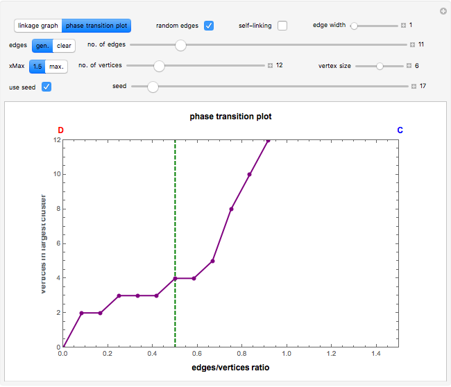
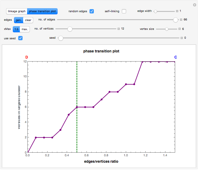
This Demonstration allows the connection of a graph of  vertices (nodes) by edges (links) drawn in either orderly or random fashion to illustrate how the graph undergoes a transition between two states, D and C, where D is a disconnected set of individual vertices and C is a single connected cluster of all the vertices. Edges are undirected and node locations are unimportant, but they are placed at the vertices of a regular -gon to simplify the drawing. Since no additional properties are assumed, the change of state from D to C can be interpreted as an abstract phase transition based solely on connectivity. Regardless of the number of vertices and edges drawn, when the number of vertices in the largest connected cluster is plotted against the edges-to-vertices ratio, the transition occurs around an edges-to-vertices ratio of 1/2, which is shown as a dashed green vertical line on the phase transition plot.
Contributed by: Mark D. Normand (September 2011)
Open content licensed under CC BY-NC-SA
Snapshots

Details
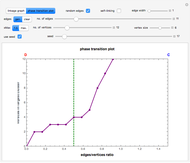
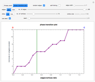
Snapshot 1: phase transition plot of the thumbnail linkage graph, where the edges/vertices ratio ( axis) maximum = 1.5
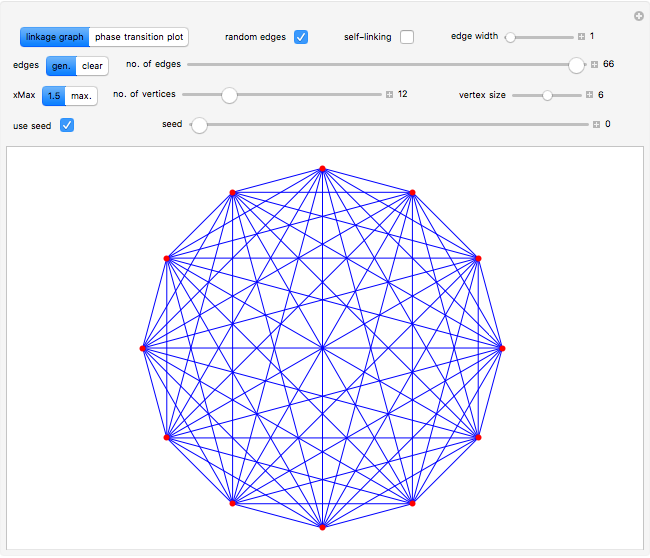
Snapshot 2: linkage graph with edges drawn randomly from seed = 0; this complete graph has  vertices and 66 edges, the maximum possible number of edges connecting 12 vertices when self-linking is not allowed
Snapshot 3: phase transition plot of the snapshot 2 linkage graph, where the edges/vertices ratio ( axis) maximum = 1.5
Snapshot 4: complete linkage graph of  vertices and 465 edges with the edges drawn randomly from seed = 17 with self-linking allowed
Snapshot 5: phase transition plot of the snapshot 4 linkage graph, where the edges/vertices ratio ( axis) maximum = 15.5, the maximum needed for 465 edges/30 vertices
Snapshot 6: linkage graph with edges drawn in nonrandom order having vertices and 11 edges; notice that  is the minimum number of edges that can link all the vertices into a single connected cluster when self-linking is not allowed
Snapshot 7: phase transition plot of the snapshot 6 linkage graph, where the edges/vertices ratio ( axis) maximum = 1.5
This Demonstration shows the connection of vertices (nodes) by edges (links) as a general model of phase transition based on connectivity according to a model described by Kauffman in [3], originally introduced by Gilbert in [2], and elaborated by Erdős and Rényi in [1]. The transition is displayed as a linkage graph of equidistant vertices marked along a circle progressively connected by straight lines, and as a corresponding phase transition plot of the number of vertices in the largest linked cluster versus the number of edges/number of vertices ratio. The curve begins with all vertices in a disconnected state, D, and ends in a connected state C, where a single cluster contains all vertices. A setter lets you toggle the output display between the default "linkage graph" and the "phase transition plot".
A slider is used to choose a number of vertices, , from 2 to 50. The vertices are drawn in the linkage graph as red dots, whose size may be varied from 2 to 10 pixels by a slider. The dots are placed at the vertices of a regular -gon to simplify drawing the linkage graph.
A complete graph is formed when each vertex is connected to every other vertex by an edge. For vertices, the number of links in a complete graph when self-linking is not allowed is  and it is
  when self-linking is allowed. For vertices, only the lower-triangular portion of an
  adjacency matrix is used to record the connection between vertices if self-linking is not allowed and the main diagonal of the adjacency matrix is also used if self-linking is allowed.
A self-liked vertex (node) is one that is linked (i.e. connected to) itself. Self-linked vertices are indicated on the linkage graph by a circle drawn around the red dot representing the vertex. The circle is blue when the edges (links) are randomly generated and black when they are generated in incremental order.
The phase transition occurs around an edges-to-vertices ratio of 1/2, which is marked on the plot as a green dashed vertical line. The "xMax" setter sets the maximum value of the axis of the plot to 1.5 by default. It may be changed to the maximum value allowed for by the current number of vertices by clicking the "max." button. This is useful to visualize how few links are needed to reach the phase transition value relative to the total number of links possible in a complete graph.
If the "random edges" box is checked, edges are drawn in blue between randomly selected pairs of vertices. When unchecked, the edges are drawn in black between vertices indexed in increasing order and the "use seed" checkbox and "seed" slider are ignored. If the "self-linking" box is checked, a small circle is drawn in either blue or black around a node to indicate that it is self-linked. The width of the edge lines may be varied from 1 to 5 pixels with a slider. The "no. of edges" slider is used to specify the number of edges to be drawn. Edges are drawn immediately based on the other control settings when the "edges" setter is set to "gen." or are erased when it is set to "clear".
If both the "random edges" and "use seed" boxes are checked, a new set of edges will be drawn in blue beginning with the seed value entered with the "seed" slider. Edges then will be added or deleted each time the "no. of edges" slider's value is changed. If the displayed edges are erased by clicking "clear" while the seed value is unchanged, exactly the same edges will be drawn again, and in exactly the same order, when "gen." is clicked. To draw a different set of randomly selected edges keeping all other settings the same, change the "seed" slider to a new value. If the "use seed" box is unchecked, any change in any control will generate a new set of randomly chosen edges drawn according to the settings of all the other controls.
References
[1] P. Erdős and A. Rényi, "On the Evolution of Random Graphs," Publ. Math. Inst. Hung. Acad. Sci., 5, 1960 pp. 17–61.
[2] E. N. Gilbert, "Random Graphs," Annals of Mathematical Statistics, 30, 1959 pp. 1141–1144.
[3] S. Kauffman, At Home in the Universe, New York: Oxford University Press, 1995 pp. 54–58.
[4] M. D. Normand and M. Peleg, "Kauffman's Abstract Model of Phase Transitions," Journal of Texture Studies, 29, 1998 pp. 375–386.
Permanent Citation
 Graph Connectivity Drawing with Four Simple Graphs
John Cicilio Cone-Based Graphs
Mirela Damian, Kelly Gremban, and Naresh Nelavalli Variations on State Transition Diagrams of Elementary Cellular Automata
Daniel de Souza Carvalho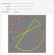 Hamilton-Connected Harary Graphs
Stan Wagon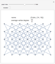 Average Vertex Degree of Connected Graphs
John Cicilio Planar Three-Connected Trivalent Network Mobile Automaton
Tommaso Bolognesi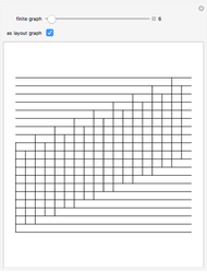 Graph Connectivity Drawing with Some Finite Graphs
John Cicilio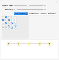 N-Step Transition Matrices for Markov Chains
Phillip Bonacich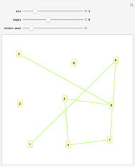 Connected Components
Ed Pegg and Daniel Lichtblau Nearest Neighbor Graph Connections
Jim Gerdy
-
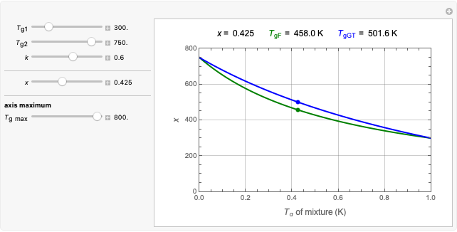 Gordon-Taylor and Fox Equations for Glass Transition Temperature
Mark D. Normand -
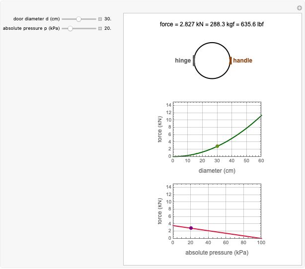 Force to Overcome Vacuum Pull
Mark D. Normand -
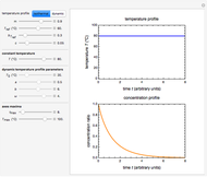
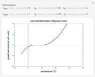 Extending the Square Root Growth Rate Model to Lethal Low Temperatures
Mark D. Normand -
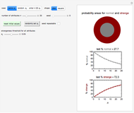 Probability of Being Strange According to Paulos
Mark D. Normand -
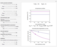
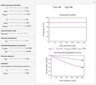
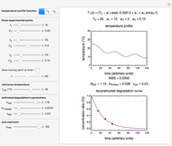 Successive Three-Point Method for Weibullian Chemical Degradation
Mark D. Normand -
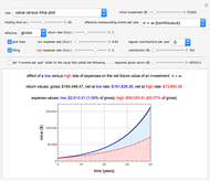 Effect of High Expense Charges on an Investment's Net Return
Mark D. Normand -
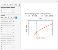 Estimating Cohesion and Tensile Strength of Compacted Powders
Mark D. Normand -
 Three-Endpoints Method for Isothermal Weibullian Chemical Degradation
Mark D. Normand -
 Vitamin C Loss in Foods During Heat Processing and Storage
Mark D. Normand -
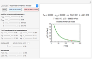 Parameterizing Temperature-Viscosity Relations
Mark D. Normand -
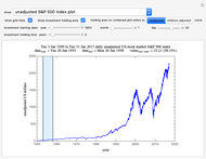 Fate of a Long-Term Index Fund Investment According to the S&P 500
Mark D. Normand -
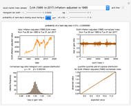 Laplace Distribution in Fluctuating Stock Index Records
Mark D. Normand -
 Weibullian Chemical Degradation
Mark D. Normand -
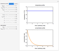 Simulating Ascorbic Acid Degradation
Mark D. Normand -
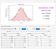 Additive and Multiplicative Risks
Mark D. Normand -
 Endpoints Method for Predicting Chemical Degradation in Frozen Foods
Mark D. Normand -
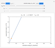 Exponential Model for Arrhenius Activation Energy
Mark D. Normand -
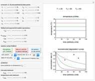
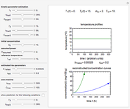
 Prediction of Isothermal Degradation by the Endpoints Method
Mark D. Normand -
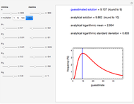 Risk Guesstimation from Factor Ranges
Mark D. Normand -
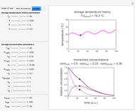
 Volatiles Formation Kinetics in Stored Fish
Mark D. Normand