Probability of Being Strange According to Paulos


Requires a Wolfram Notebook System
Interact on desktop, mobile and cloud with the free Wolfram Player or other Wolfram Language products.
In his short autobiographical book, entitled A Numerate Life: A Mathematician Explores the Vagaries of Life, His Own and Probably Yours (2015), John Allen Paulos [1] demonstrates that most people, even ordinary-looking ones, are probably "strange." If "strangeness" is defined as having an attribute (trait) that is at either end of its distribution in a human population (e.g. being at the top or bottom 5% of an adult's height), then if an individual is judged by several independent attributes, the probability of remaining "normal" decreases rapidly as the number of considered attributes is increased.
[more]
Contributed by: Mark D. Normandand Micha Peleg (April 2018)
Open content licensed under CC BY-NC-SA
Snapshots


Details
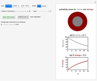
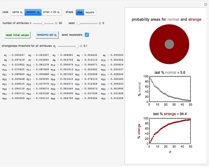
Snapshot 1: normality and strangeness determined by 100 attributes with fixed boundaries 
Snapshot 2: normality and strangeness determined by 50 attributes with randomly chosen individual boundaries
Snapshot 3: normality and strangeness determined by 20 attributes with manually chosen individual boundaries
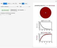
Snapshot 4: normality and strangeness determined by 40 attributes with randomly chosen individual boundaries and showing a square probability area display
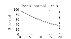
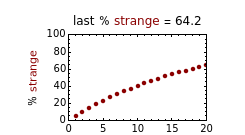
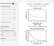
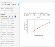
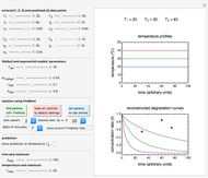
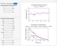
According to Paulos [1], strangeness can be defined as being beyond the range considered normal. Assuming for simplicity that a chosen attribute is uniformly distributed, being strange can be defined as being at the top or bottom 5%, for example; then the probability of being normal is  or 90% and of being strange is 0.1 or 10%. When a person's normality or strangeness is determined by two attributes, with the same 5% criterion, then the probability of encountering a normal person drops to 0.81 or 81%. For three attributes, it drops to 0.729 or 72.9%; for four attributes it drops to 0.656 or 65.6%; and so on. For 50 attributes, the probability of encountering a normal person drops to 0.515%, and for 100 attributes to only 0.00266%.
Where the strangeness criterion is the same for all the attributes, as in the given example, the probability of encountering a normal person when judged by  attributes, that is, by vectors in an -dimensional space, is calculated with the formula
  , where
  is the total fraction of the extremes in each of the attributes,
  as in the given example.
For the more general case where the strangeness criterion is allowed to vary among the attributes (and need not be symmetric), the percent probability of encountering a normal person is calculated by the formula 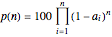 .
.
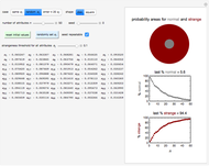
This Demonstration provides visualization of the increasing strangeness and correspondingly diminishing normality in two graphical forms as chosen by the user: (1) a dark red ring whose variable area represents the strangeness probability surrounding a gray disk whose area represents the probability of normality, or (2) a dark red square frame whose variable area represents the strangeness probability surrounding a gray square whose area represents the probability of normality.
This Demonstration plots the increasing probability of strangeness and the diminishing probability of normality as functions of from 1 to a maximum of 100 and displays their (last) numerical values for the chosen in dark red and gray, respectively, above each plot.
The attributes' threshold values can all be the same, determined by the  slider, if the first setter (case 1: "same ") is checked. It can be varied randomly within a chosen range (case 2: "random "), in which case the number (from 1 to 100) of attributes' actual values will be displayed. A third option (case 3: "enter
 ") allows for manually entering the values of up to 20 attributes, each with its own slider.
For case 2, each time the blue "randomly set " setter is clicked, a new random set of values is generated. If the "seed repeatable" box is checked, the same set of random values for all attributes is generated from the value set by the "seed" slider. The initial default settings of all controls may be restored by clicking the green "reset initial values" button.
Notice that this Demonstration only provides a visualization of the general concept using the simplest uniform distribution function, without making any attempt to identify actual attributes and their thresholds.
Reference
[1] J. A. Paulos, A Numerate Life: A Mathematician Explores the Vagaries of Life, His Own and Probably Yours, Amherst, NY: Prometheus Books, 2015.
Permanent Citation
 Probability of Being Sick After Having Tested Positive for a Disease (Bayes's Rule)
Frank Scherbaum Stock Price Probability with Stable Distributions
Bob Rimmer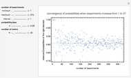 Convergence of Probability II: Condorcet's Jury Theorem, Part 4
Tetsuya Saito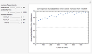 Convergence of Probability I: Condorcet's Jury Theorem, Part 3
Tetsuya Saito Closed-Form Full Life Cycle Distribution
Kelly S. Lowder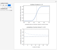 Theoretical Model: Condorcet's Jury Theorem, Part 1
Tetsuya Saito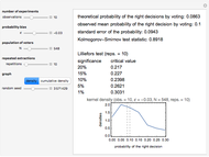 Kernel Density Estimations: Condorcet's Jury Theorem, Part 5
Tetsuya Saito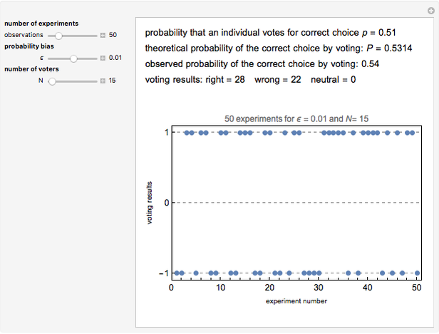 Vote for Justice: Condorcet's Jury Theorem, Part 2
Tetsuya Saito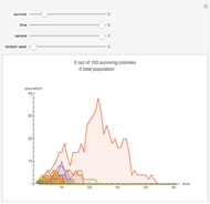 An Amoeba Problem
Jason Cawley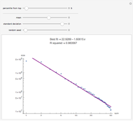 Power Law Tails in Log Normal Data
Fiona Maclachlan
-
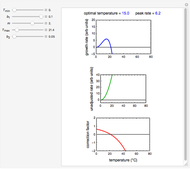 Ratkowski's Square Root Growth Rate Model for High Temperatures
Micha Peleg -
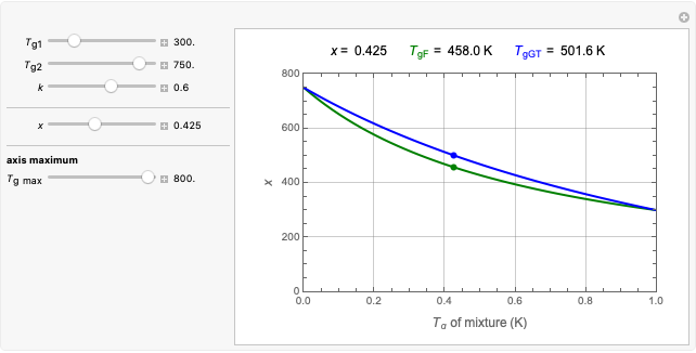 Gordon-Taylor and Fox Equations for Glass Transition Temperature
Micha Peleg -
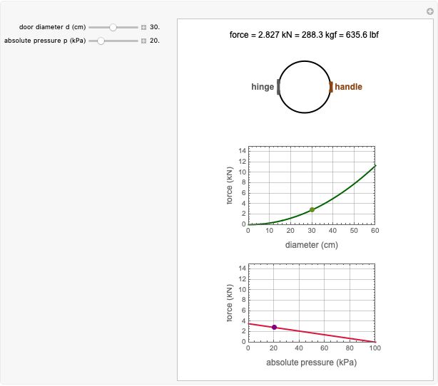 Force to Overcome Vacuum Pull
Micha Peleg -
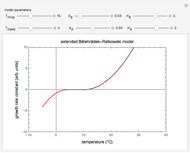 Extending the Square Root Growth Rate Model to Lethal Low Temperatures
Micha Peleg -
 Probability of Being Strange According to Paulos
Micha Peleg -
 Successive Three-Point Method for Weibullian Chemical Degradation
Micha Peleg -
 Estimating Cohesion and Tensile Strength of Compacted Powders
Micha Peleg -
 Three-Endpoints Method for Isothermal Weibullian Chemical Degradation
Micha Peleg -
 Vitamin C Loss in Foods During Heat Processing and Storage
Micha Peleg -
 Parameterizing Temperature-Viscosity Relations
Micha Peleg -
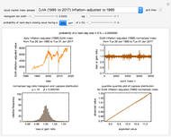 Laplace Distribution in Fluctuating Stock Index Records
Micha Peleg -
 Weibullian Chemical Degradation
Micha Peleg -
 Simulating Ascorbic Acid Degradation
Micha Peleg -
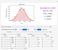 Additive and Multiplicative Risks
Micha Peleg -
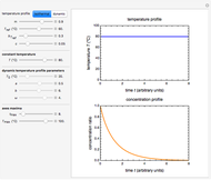
 Endpoints Method for Predicting Chemical Degradation in Frozen Foods
Micha Peleg -
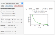
 Exponential Model for Arrhenius Activation Energy
Micha Peleg -
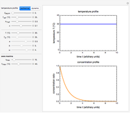
 Prediction of Isothermal Degradation by the Endpoints Method
Micha Peleg -
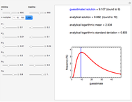 Risk Guesstimation from Factor Ranges
Micha Peleg -
 Volatiles Formation Kinetics in Stored Fish
Micha Peleg -
 Comparison of Six Sigmoid Growth Curve Models
Micha Peleg