Three-Endpoints Method for Isothermal Weibullian Chemical Degradation


Requires a Wolfram Notebook System
Interact on desktop, mobile and cloud with the free Wolfram Player or other Wolfram Language products.
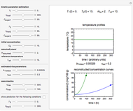
Consider the degradation of a heat-labile compound during isothermal storage or exposure to a high constant temperature. Assume that this process follows Weibull kinetics. If the temperature dependence of the rate parameter follows the exponential model, a simpler alternative to the Arrhenius equation, then the compound's diminishing concentration is specified by three kinetic parameters. These can be extracted from three concentration ratios determined at three different constant temperatures at the same or at different times.
[more]
Contributed by: Mark D. Normand and Micha Peleg (September 2017)
Open content licensed under CC BY-NC-SA
Snapshots
Details
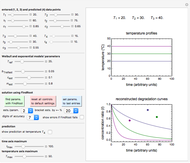
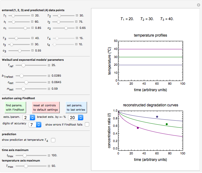
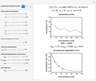
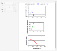
Snapshot 1: entered data points with the default parameter settings
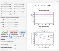
Snapshot 2: the data points shown in Snapshot 1 approximately matched visually with their corresponding reconstructed degradation curves; note the kinetic parameter sliders' positions
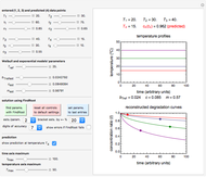
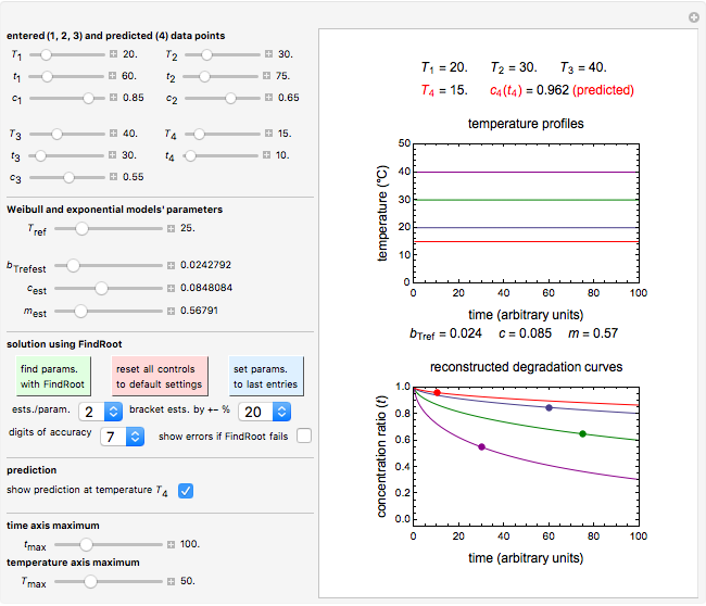
Snapshot 3: using the approximate match shown in Snapshot 2 to calculate the kinetic parameters using FindRoot and predicting the curve at a fourth temperature; note the kinetic parameter sliders' new positions
Snapshot 4: isothermal ambient degradation pattern predicted (red curve and point) from accelerated storage data using a visual match of the other curves to the three entered points
Snapshot 5: isothermal degradation at a high temperature predicted (red curve and point) from lower temperature data using a visual match of the other curves to the three entered points
Many, perhaps most, degradation reactions follow first-order kinetics, at least as a first approximation, and occasionally other fixed-order kinetics. Nevertheless, first-order degradation can be viewed as a special case of the Weibull model where the shape factor is equal to 1. The Weibull model for isothermal decay can be written in the form
 ,
,
where 
is the momentary concentration ratio at time  ,
,  is a temperature-dependent rate parameter (related to the scale factor in the Weibull distribution), and
  is a concavity parameter (the shape factor in the Weibull distribution), usually a constant or very weakly varying function of temperature [1].
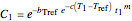
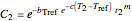
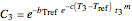
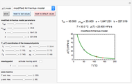
Traditionally, the temperature dependence of the rate constant of chemical reactions has been described by the Arrhenius equation. It has been demonstrated that at pertinent temperatures the Arrhenius equation can be replaced by the simpler exponential model [2], which when applied to the Weibullian model's rate parameter assumes the form
where  is the magnitude of at a chosen reference temperature
  , and
, and  is a temperature sensitivity parameter expressed in
  units. Combining the two equations renders the isothermal Weibullian-exponential model
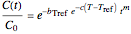 .
.
Conventionally, kinetic degradation parameters have been determined from a set of experimental isothermal concentration versus time relationships at several constant temperatures. To reduce the associated logistic load, it has been proposed to use the endpoints method whereby these parameters are estimated from a much smaller number of selected points [3]. For our purpose, this translates to the following: consider three concentration ratios  ,
,  and
and  determined after times
  ,
,  and
and  at temperatures
  ,
,  and
and  , respectively. If the Weibullian-exponential model holds, then for any chosen we have three simultaneous equations
 ,
,
 and
and
 ,
,
with ,  and
and  the three unknowns.
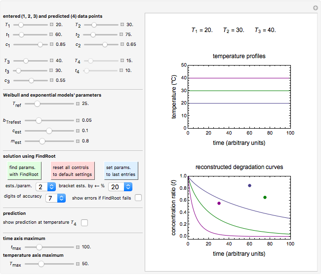
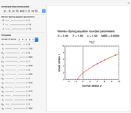
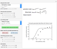
Being nonlinear, these equations require numerical solution, which, in turn, requires proper initial values for the FindRoot function to determine a solution. Obtaining these initial values by trial and error can be a daunting task, and a solution for experimentally determined concentrations is not always guaranteed. This Demonstration offers a convenient and rapid way to estimate the kinetic parameters and/or find initial values for their numerical calculation. This is done by generating three reconstructed degradation curves using , and values obtained by moving sliders on the screen until they match or approximately match the three entered (experimental) points. Once a match is obtained, the parameter slider's positions provide an estimate of their values. They can also be used as entered or multiplied by two factors, 0.8 and 1.2, for example, as the starting point or points for the FindRoot function to calculate the , and values that produce the best match. These estimated or calculated parameter values are then used to reconstruct the entire degradation curves for the temperatures , and and to predict the concentration at any chosen temperature  not used in determining the parameters, assuming that the model holds at that temperature.
To start, enter the three points, using their corresponding sliders at the top left of the panel. Then choose the reference temperature and move the , and sliders until a visual match is obtained between the three reconstructed curves and the three entered data points. Before or when this is accomplished, you can click the "find params. with FindRoot" setter to find the numerical solution of the three equations. If successful, the corresponding values of the parameters will be displayed between the plots and next to their sliders. Notice that for some entries FindRoot can find a solution even with the default parameter values, while for others no solution is possible.
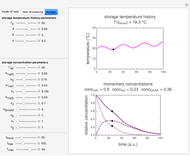
To choose a fourth temperature, click the "show prediction at temperature " checkbox to display the predicted degradation curve for that temperature, which will appear in red. This will also activate the and  sliders, which can then be used to calculate the concentration ratio at a chosen time and plot it on the predicted degradation curve. The numerical values of the chosen and corresponding concentration ratio will be displayed in red above the temperature plot and can be used to validate the model by comparing the prediction with an actual concentration.
Use the lower two sliders to adjust the plot time and temperature axes maxima.
Notice that not all allowed entries have a numerical solution, in which case the message "No solution with current entries." will appear in red. This, or failure to match the reconstructed curves, can be caused by errors in the entered data and/or the particular degradation reaction not following the assumed kinetic model.
References
[1] M. A. J. S. van Boekel, Kinetic Modeling of Reactions in Foods, Boca Raton: CRC Press, 2009.
[2] M. Peleg, M. D. Normand and M. G. Corradini, "The Arrhenius Equation Revisited," Critical Reviews in Food Science and Nutrition, 52(9), 2012 pp. 830–851. doi:10.1080/10408398.2012.667460.
[3] M. Peleg, M. D. Normand and M. G. Corradini, "A New Look at Kinetics in Relation to Food Storage," Annual Review of Food Science and Technology, 8(1), 2017 pp. 135–153. doi:10.1146/annurev-food-030216-025915.
Permanent Citation
 Successive Three-Point Method for Weibullian Chemical Degradation
Mark D. Normand and Micha Peleg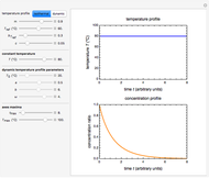 Weibullian Chemical Degradation
Mark D. Normand and Micha Peleg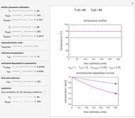 Prediction of Isothermal Degradation by the Endpoints Method
Mark D. Normand and Micha Peleg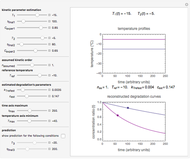 Endpoints Method for Predicting Chemical Degradation in Frozen Foods
Mark D. Normand and Micha Peleg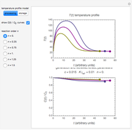 Extracting Fixed-Order Degradation Kinetics by the Endpoints Method
Mark D. Normand and Micha Peleg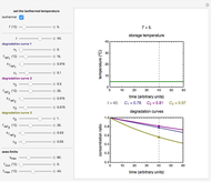 Thermal Degradation of Three Nutrients in Foods
Mark D. Normand and Micha Peleg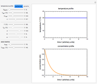 Simulating Ascorbic Acid Degradation
Mark D. Normand and Micha Peleg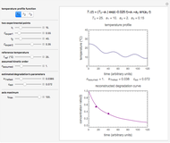 Degradation Parameters from Concentration Ratios
Mark D. Normand and Micha Peleg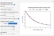 Fit of First-Order Kinetic Model in Degradation Processes
Mark D. Normand and Micha Peleg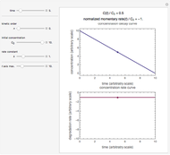 Kinetic Order of Degradation Reactions
Mark D. Normand and Micha Peleg
-
 Ratkowski's Square Root Growth Rate Model for High Temperatures
Micha Peleg -
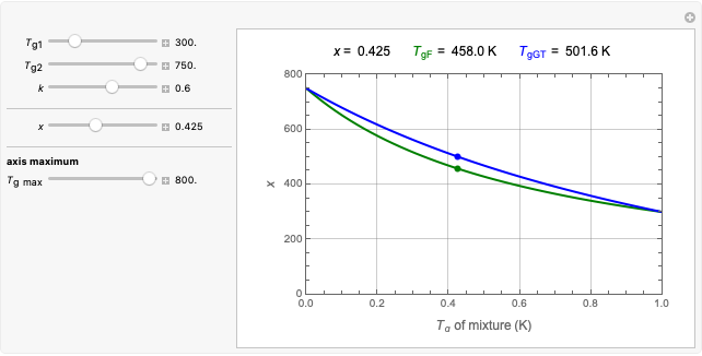 Gordon-Taylor and Fox Equations for Glass Transition Temperature
Micha Peleg -
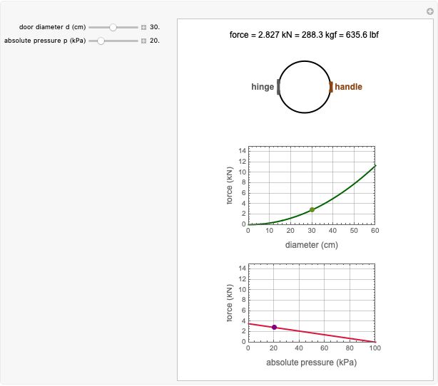 Force to Overcome Vacuum Pull
Micha Peleg -
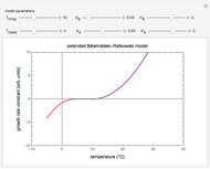 Extending the Square Root Growth Rate Model to Lethal Low Temperatures
Micha Peleg -
 Probability of Being Strange According to Paulos
Micha Peleg -
Successive Three-Point Method for Weibullian Chemical Degradation
Micha Peleg -
 Estimating Cohesion and Tensile Strength of Compacted Powders
Micha Peleg -
 Three-Endpoints Method for Isothermal Weibullian Chemical Degradation
Micha Peleg -
 Vitamin C Loss in Foods During Heat Processing and Storage
Micha Peleg -
 Parameterizing Temperature-Viscosity Relations
Micha Peleg -
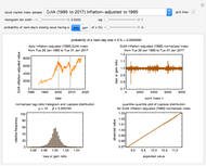 Laplace Distribution in Fluctuating Stock Index Records
Micha Peleg -
Weibullian Chemical Degradation
Micha Peleg -
Simulating Ascorbic Acid Degradation
Micha Peleg -
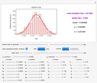 Additive and Multiplicative Risks
Micha Peleg -
Endpoints Method for Predicting Chemical Degradation in Frozen Foods
Micha Peleg -
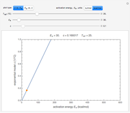 Exponential Model for Arrhenius Activation Energy
Micha Peleg -
Prediction of Isothermal Degradation by the Endpoints Method
Micha Peleg -
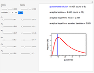 Risk Guesstimation from Factor Ranges
Micha Peleg -
 Volatiles Formation Kinetics in Stored Fish
Micha Peleg -
 Comparison of Six Sigmoid Growth Curve Models
Micha Peleg