Weibullian Chemical Degradation

Requires a Wolfram Notebook System
Interact on desktop, mobile and cloud with the free Wolfram Player or other Wolfram Language products.
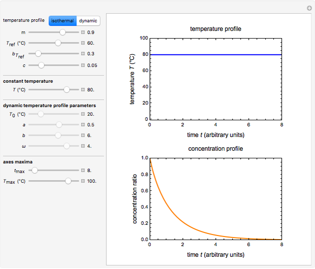
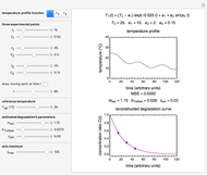
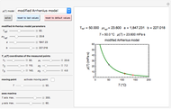
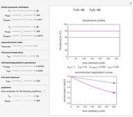
This Demonstration shows isothermal and selected dynamic chemical degradation patterns that follow the Weibullian ("stretched exponential") model with a constant shape factor (exponent). The temperature dependence of the rate parameter is described by a simple exponential model which, as has been previously shown, can be used interchangeably with the Arrhenius equation.
Contributed by: Mark D. Normandand Micha Peleg (September 2016)
Open content licensed under CC BY-NC-SA
Snapshots
Details
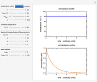
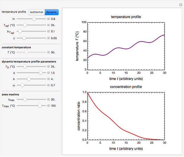
Snapshot 1: isothermal degradation curve following the Weibullian model
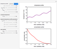
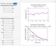
Snapshot 2: nonisothermal degradation curve following the Weibullian model (rising oscillating temperature)
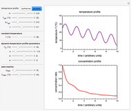
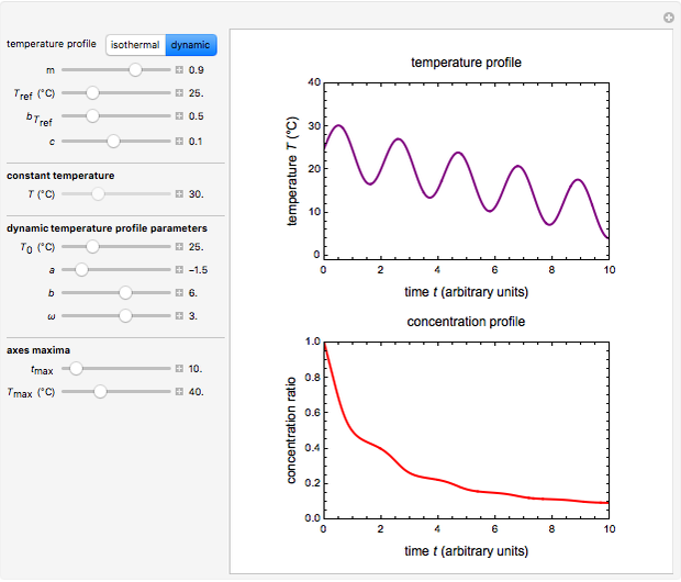
Snapshot 3: nonisothermal degradation curve following the Weibullian model (falling oscillating temperature)
There is evidence in the literature that the isothermal degradation of certain nutrients can sometimes be better described by the Weibullian model  than by fixed-order kinetics [1, 2].
  in this model is the time-dependent concentration ratio,
  is a temperature-dependent rate constant and
  is the shape factor, assumed to be constant or a very weak function of temperature.
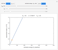
The temperature dependence of  is assumed to follow the Arrhenius equation, which can be replaced by the simpler exponential model
 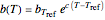 without sacrificing the fit [3]. In this model,
  is the rate constant at an arbitrary reference temperature
  , both
  and are in °C, and
  is a characteristic constant having units of
  . Incorporating , thus defined, into the isothermal degradation equation leads to the general isothermal model
 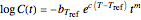 .
.
Assume that when the temperature varies, the degradation rate is the isothermal rate at temperature  , at time
  that corresponds to the concentration ratio [2, 4]. Implementing this assumption renders the general dynamic degradation model in the form
  , with the boundary condition
  , from which
  is determined.
In this Demonstration you can choose between simulating isothermal degradation at chosen constant temperatures or, as examples, dynamic degradation at linearly rising and falling oscillating temperatures. You can vary the degradation kinetic parameters, namely, , and with sliders. You can also vary the constant temperature . For dynamic degradation, you can vary the temperature profile parameters  , the initial temperature
  in °C, the slope of the temperature rise
  or fall
  in
in  units, the temperature oscillation amplitude
  in °C, and the frequency
  in units of
  .
.
Not all combinations of the temperature profile parameters , , and in the dynamic temperature profile equation and the kinetic parameters , and lead to realistic degradation curves.
References
[1] M. G. Corradini and M. Peleg, "A Model of Non-isothermal Degradation of Nutrients, Pigments and Enzymes," Journal of the Science of Food and Agriculture, 84(3), 2004 pp. 217–226. doi:10.1002/jsfa.1647.
[2] M. G. Corradini and M. Peleg, "Prediction of Vitamins Loss During Non-isothermal Heat Processes and Storage with Non-linear Kinetic Models," Trends in Food Science and Technology, 17(1), 2006 pp. 24–34. doi:10.1016/j.tifs.2005.09.004.
[3] M. Peleg, M. D. Normand and M. G. Corradini, "The Arrhenius Equation Revisited," Critical Reviews in Food Science and Nutrition, 52(9), 2012 pp. 830–851. doi:10.1080/10408398.2012.667460.
[4] M. Peleg, A. D. Kim and M. D. Normand, "Predicting Anthocyanins' Isothermal and Non-isothermal Degradation with the Endpoints Method," Food Chemistry, 187(15), 2015 pp. 537–544. doi:10.1016/j.foodchem.2015.04.091.
Permanent Citation
 Successive Three-Point Method for Weibullian Chemical Degradation
Mark D. Normand and Micha Peleg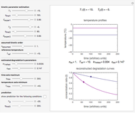 Endpoints Method for Predicting Chemical Degradation in Frozen Foods
Mark D. Normand and Micha Peleg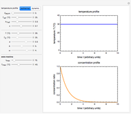 Simulating Ascorbic Acid Degradation
Mark D. Normand and Micha Peleg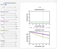 Thermal Degradation of Three Nutrients in Foods
Mark D. Normand and Micha Peleg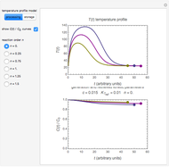 Extracting Fixed-Order Degradation Kinetics by the Endpoints Method
Mark D. Normand and Micha Peleg Eyring-Polanyi versus Exponential Model for Chemical Reactions
Mark D. Normand, Christina S. Barsa, and Micha Peleg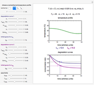 Determining Shelf Life by Two Criteria
Mark D. Normand and Micha Peleg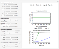 Volatiles Formation Kinetics in Stored Fish
Mark D. Normand and Micha Peleg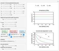 Three-Endpoints Method for Isothermal Weibullian Chemical Degradation
Mark D. Normand and Micha Peleg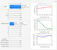 Nonisothermal Degradation Kinetics
Mark D. Normand and Micha Peleg
-
 Ratkowski's Square Root Growth Rate Model for High Temperatures
Micha Peleg -
 Gordon-Taylor and Fox Equations for Glass Transition Temperature
Micha Peleg -
 Force to Overcome Vacuum Pull
Micha Peleg -
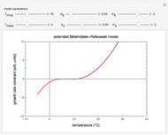 Extending the Square Root Growth Rate Model to Lethal Low Temperatures
Micha Peleg -
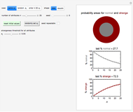 Probability of Being Strange According to Paulos
Micha Peleg -
Successive Three-Point Method for Weibullian Chemical Degradation
Micha Peleg -
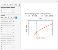 Estimating Cohesion and Tensile Strength of Compacted Powders
Micha Peleg -
Three-Endpoints Method for Isothermal Weibullian Chemical Degradation
Micha Peleg -
 Vitamin C Loss in Foods During Heat Processing and Storage
Micha Peleg -
 Parameterizing Temperature-Viscosity Relations
Micha Peleg -
 Laplace Distribution in Fluctuating Stock Index Records
Micha Peleg -
 Weibullian Chemical Degradation
Micha Peleg -
Simulating Ascorbic Acid Degradation
Micha Peleg -
 Additive and Multiplicative Risks
Micha Peleg -
Endpoints Method for Predicting Chemical Degradation in Frozen Foods
Micha Peleg -
 Exponential Model for Arrhenius Activation Energy
Micha Peleg -
 Prediction of Isothermal Degradation by the Endpoints Method
Micha Peleg -
 Risk Guesstimation from Factor Ranges
Micha Peleg -
Volatiles Formation Kinetics in Stored Fish
Micha Peleg -
 Comparison of Six Sigmoid Growth Curve Models
Micha Peleg