Exact and Approximate Relativistic Corrections to the Orbital Precession of Mercury


Requires a Wolfram Notebook System
Interact on desktop, mobile and cloud with the free Wolfram Player or other Wolfram Language products.
Accounting for the anomaly in the perihelion precession of Mercury provided early support for Einstein's General Theory of Relativity [1]. Very conveniently, accurate astronomical data was already available. Schwarzschild's solution to Einstein's gravitational field equations can be approximated by Newtonian gravity perturbed by a short-range term of magnitude proportional to the Schwarzschild radius  , where
  is the universal gravitational constant,
  is the attracting mass (the Sun) and
  is the speed of light [2, 3].


Contributed by: Brad Klee. (September 2016)
Open content licensed under CC BY-NC-SA
Details
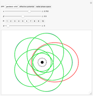
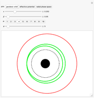
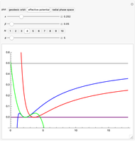
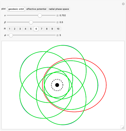
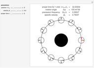
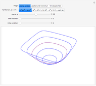
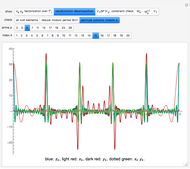
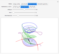
In all plots, blue shows the exact solution, green shows the arbitrary-precision approximation and red shows the classical Kepler/Newton approximation.
In this computation, we set  and
and  . Then the effective radial potential is:

with minimum at
 ,
,
where we introduce the normalized parameter

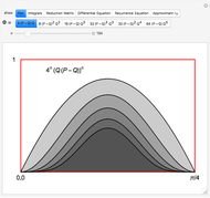
restricted to the range  . Expanding the potential around the minimum gives

with
 .
.
The frequency  of small oscillations is then given by
 .
.
Taking the first-order term from the Big Precession Equation (see Estimating Planetary Perihelion Precession) and substituting in values for  , we obtain [8]:
 .
.
This is the simplest exact form for zero-order precession. As  and
and  , then
  and there is no precession. As
  and
and  , then
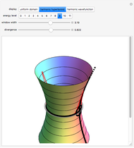
  . In terms of the effective potential, the divergence occurs as the local minimum nears the local maximum and the curve flattens out. The local max and min coincide when
  . The Schwarzschild radius is at
  . At the critical point,
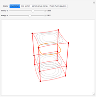
  gives the relative radius of the innermost stable circular orbit (isco), depicted as a dashed black line around the black hole in the orbit graphs. The prediction that
  provides a test for all solutions: as
  , the orbit should approach no closer to
  than
than  .
.
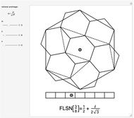
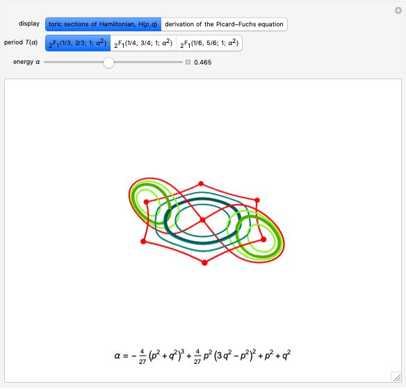
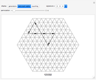
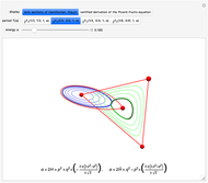
Other authors [9-11] discuss aesthetically pleasing solutions that arise from a conspiracy of parameters, as occurs with  ,
,  . It is possible to write an algorithm that operates on the approximate solution, a particular value for
  and a rational number
  ,
,  , that returns an approximate solution for the
  value, ultimately by finding the root of a polynomial equation. Acceptable values close to
  can be found quickly using a linear procedure because

is a small number. For example for  and
and  ,
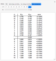
,  . Doing a quick search, we obtain the following approximate "Magic Numbers":
$Failed
Exploring these sequences shows interesting properties of closed orbits. We see that each figure has  -fold dihedral symmetry with
  crossing points.
From a mathematical perspective, it would be interesting to extend the precision measurement of  values, prove the empirical crossing formula and give a physical characterization of the crossing points using the full equations of motion, but physicists will be more interested in comparing predictions with data. Planetary precession calculations often use only the zero-order precession terms. For example, Mercury has
 ,
,
 ,
,
which implies
 arcseconds per Julian century.
Substituting  , this Demonstration shows that a Kepler/Newton approximation is almost good enough to describe an isolated Mercury-Sun system on the order of one year. In more extreme gravity, the zero-order approximation fails, and higher-order energy dependence needs to be considered. This is an exciting opportunity, as humankind continues to develop incredible new experiments in black hole astronomy [2, 6].
References
[1] A. Einstein, "Erklärung der Perihelionbewegung der Merkur aus der allgemeinen Relativitätstheorie." Sitzungsberichte der Königlich Preußischen Akademie der Wissenschaften, 1915 pp. 831–839. (Sep 27, 2016) einsteinpapers.press.princeton.edu/vol6-doc/261. English translation: einsteinpapers.press.princeton.edu/vol6-trans/128?ajax.
[2] J. A. Wheeler, A Journey into Gravity and Spacetime, New York: W. H. Freeman and Co., 1990 pp. 168–183.
[3] R. M. Wald, General Relativity, Chicago: University of Chicago Press, 1984 pp. 139–143.
[4] K. Weierstrass, "Zur Theorie der elliptischen Functionen," Sitzungsberichte der Königlich Preußischen Akademie der Wissenschaften, 1882. (Sep 28, 2016) archive.org/stream/mathematischewer02weieuoft#page/244/mode/2up.
[5] M. Abramowitz and I. A. Stegun (eds.), Handbook of Mathematical Functions with Formulas, Graphs, and Mathematical Tables, New York: Dover Publications, 1965. (Sep 28, 2016) people.math.sfu.ca/~cbm/aands/page_627.htm.
[6] G. Scharf. "Schwarzschild Geodesics in Terms of Elliptic Functions and the Related Red Shift." arxiv.org/abs/1101.1207.
[7] B. Klee. "Plane Pendulum and Beyond by Phase Space Geometry." arxiv.org/abs/1605.09102.
[8] F. Frohlich. "Another Planetary Sequence" (thread). SeqFan. (Sep 11, 2016) list.seqfan.eu/pipermail/seqfan/2016-September/016731.html.
[9] P. Erdös, "Spiraling the Earth with C. G. J. Jacobi," American Journal of Physics, 68(10), 2000 pp. 888–895. doi:10.1119/1.1285882.
[10] W. G. Harter. "Classical Mechanics with a Bang!," Unit 3, p. 46. (Sep 28, 2016) www.uark.edu/ua/modphys/markup/CMwBang_Info_ 2016.html.
[11] S. Wolfram, "Black Hole Tech?," from Stephen Wolfram Blog—A Wolfram Web Resource. (Sep 28, 2016) blog.stephenwolfram.com/2016/02/black-hole-tech.
Snapshots


Permanent Citation
 Geodesic Precession on a Timelike Circular Orbit around a Schwarzschild Black Hole
Thomas Müller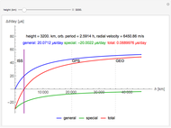 Relativistic Effects on Satellite Clock as Seen from Earth
Jakub Serych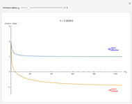 Effective and Inertial Masses of a Photon Near a Black Hole for a Family of Envelope Orbits
Wladimir Belayev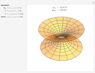 Geodesics in the Morris-Thorne Wormhole Spacetime
Thomas Müller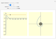 Geodesics in Schwarzschild Space
Niels Walet Estimating Planetary Perihelion Precession
Brad Klee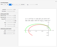 The Gravitational Two-Body Problem in the Einstein-Infeld-Hoffmann Approximation
Ulrich Mutze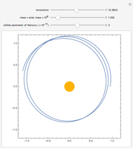 Mercury's Perihelion Precession
Enrique Zeleny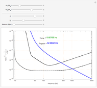 Gravitational Waves from Non-precessing Spinning Binary Black Hole Coalescence
Satya Mohapatra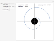 Orbits around Schwarzschild Black Holes
David Saroff
-
 Exact and Approximate Relativistic Corrections to the Orbital Precession of Mercury
Brad Klee -
 Algebraic Family of Trefoil Curves
Brad Klee -
 Kermack-McKendrick SIR Model
Brad Klee -
 Summer Insect Pandemics in the United States
Brad Klee -
 Molien Series for a Few Double Groups
Brad Klee -
 Flowsnake Q-Function
Brad Klee -
 Edwards's Solution of Pendulum Oscillation
Brad Klee -
 A Family of NxN Space-Filling Z-Functions, N>1
Brad Klee -
 Semiclassical Quantization for Asymmetric Rigid Rotors
Brad Klee -
 A Few More Geometries after Ramanujan
Brad Klee -
 Code 686 Builds the Chair Tiling
Brad Klee -
 Semiclassical Approximation for Quantum Harmonic Oscillator Wavefunctions
Brad Klee -
 Multipole Expansions of Electric Fields
Brad Klee -
 D4 Symmetric Stratum of Quartic Plane Curves
Brad Klee -
 Factoring the Even Trigonometric Polynomials of A269254
Brad Klee -
 Approximating Pi with Trigonometric-Polynomial Integrals
Brad Klee -
 Four Hypergeometric Lattice Walks
Brad Klee -
 Deriving Hypergeometric Picard-Fuchs Equations
Brad Klee -
 Discrete and Continuous Quartic Anharmonic Oscillation
Brad Klee -
 Weierstrass Solution of Cubic Anharmonic Oscillation
Brad Klee