Constant Risk Aversion Utility Functions


Requires a Wolfram Notebook System
Interact on desktop, mobile and cloud with the free Wolfram Player or other Wolfram Language products.
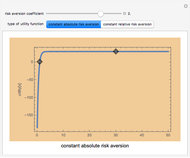
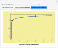
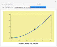
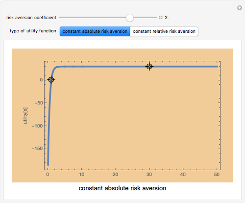
Utility functions are said to exhibit constant risk aversion under the Arrow–Pratt measure if they satisfy a secondâ€Âorder differential equation. You can set a risk aversion coefficient—the higher it is, the more risk averse—as well as the values at two points along the curve; this Demonstration plots the resulting utility function. You can choose between constant absolute risk aversion and constant relative risk aversion. The class of utility functions shown in this Demonstration are frequently used in economic analyses of risk, including finance and insurance.
Contributed by: Seth J. Chandler (March 2011)
Open content licensed under CC BY-NC-SA
Snapshots


Details
Although it appears that the locators are constrained to stay along the original curve, this is not the case: the locators are unconstrained. The fact that the curve does not change its shape is the result of constant risk aversion and the use of the  option.
Snapshot 1: a high level of constant risk aversion results in a rapid flattening of the utility function
Snapshot 2: a logarithmic utility function results when constant relative aversion is set to one
Snapshot 3: a utility function reflecting negative risk aversion
Permanent Citation
"Constant Risk Aversion Utility Functions"
http://demonstrations.wolfram.com/ConstantRiskAversionUtilityFunctions/
Wolfram Demonstrations Project
Published: March 7 2011
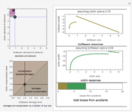 Bilateral Accident Model
Seth J. Chandler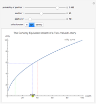 Certainty Equivalent Wealth
Seth J. Chandler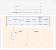 Moral Hazard
Seth J. Chandler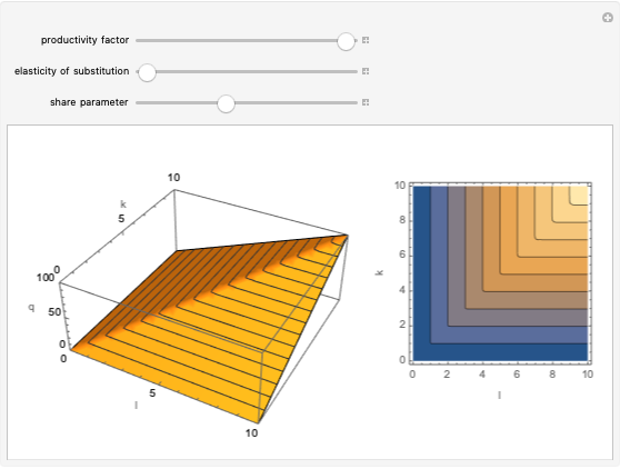 Constant Elasticity of Substitution Production
Kevin Balch and Seth J. Chandler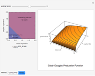 Cobb-Douglas Production Functions
Seth J. Chandler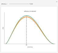 Land Use Regulation and Municipal Utility
Roger J. Brown Risk, Ownership, and Control
Roger J. Brown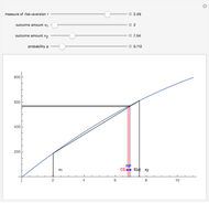 Risk Premiums
John Horton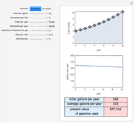 The Present Value of Future Gas Use
Seth J. Chandler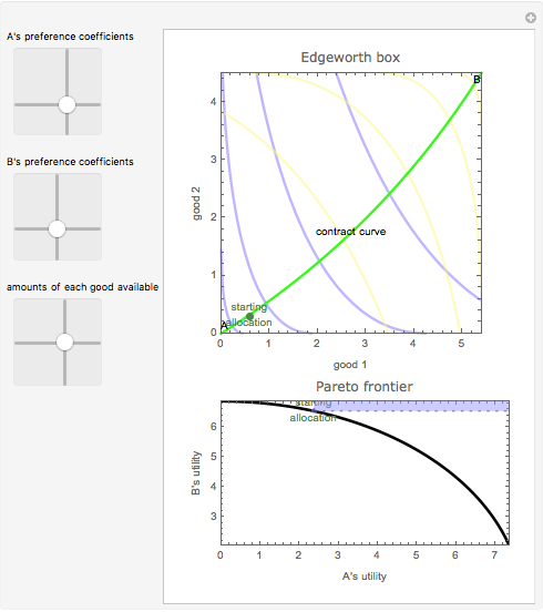 The Edgeworth Box
Seth J. Chandler
-
 Post-Event Bonding
Seth J. Chandler -
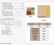
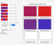 Emulating Land Use Evolution with a Cellular Automaton
Seth J. Chandler -
 General Assembly Resolution Viewer
Seth J. Chandler -
 Random Acyclic Networks
Seth J. Chandler -
 A Theory of Insurance Lapses
Seth J. Chandler -
 Asylum in the United States
Seth J. Chandler -
 Property Coinsurance
Seth J. Chandler -
 The Persuasion Effect: A Traditional Two-Stage Jury Model
Seth J. Chandler -
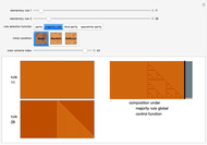 Cellular Automata with Global Control
Seth J. Chandler -
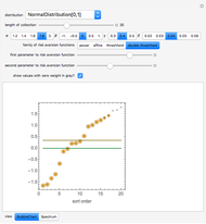
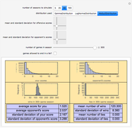 Sports Seasons Based on Score Distributions
Seth J. Chandler -
 Evidentiary Uncertainty
Seth J. Chandler -
 Spectral Measures
Seth J. Chandler -
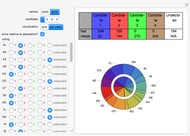 The Banzhaf Power Index of States for Presidential Candidates
Seth J. Chandler -
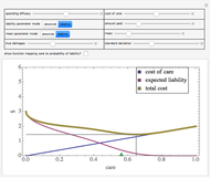
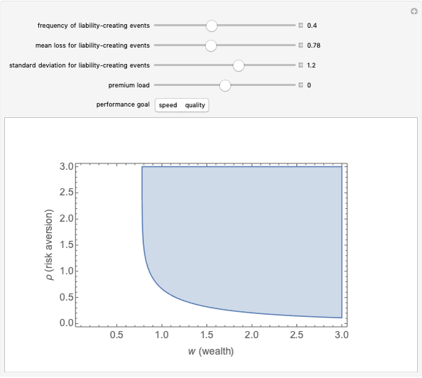 Liability Insurance Desirability under Lognormal Loss Distributions
Seth J. Chandler -
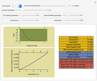 The Effects of Coinsurance and Deductibles on Optimal Precautions for Weibull-Distributed Loss
Seth J. Chandler -
 Collocation by Chi Square
Seth J. Chandler -
The Present Value of Future Gas Use
Seth J. Chandler -
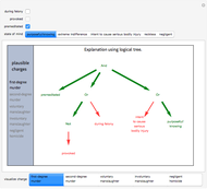 Visualizing Legal Rules: A Homicide Case
Seth J. Chandler -
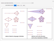 Communities of Nations Bridged by Language Similarity
Seth J. Chandler