Estimating the Local Mean Function


Requires a Wolfram Notebook System
Interact on desktop, mobile and cloud with the free Wolfram Player or other Wolfram Language products.
The linear regression model  relies on a number of crucial assumptions, the most important of which is a linear relationship between the covariate
  and the dependent variable
  . One way of generalizing the standard linear regression model is to extend it to the nonlinear form
  , where
  and
and  are real-valued functions and
  is an independent, identically distributed sequence of standard normal random variables. We study five different sets of data (three "real" and two simulated) to illustrate how kernel-weighted least-squares regression can be used to estimate the local mean function
 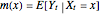 .
.
Contributed by: Jeff Hamrick (December 2008)
Open content licensed under CC BY-NC-SA
Snapshots

Details
There is an extensive literature on nonlinear regression and nonparametric estimation techniques. We refer the reader to the notable book by Fan and Yao and extensive work by Bjerve and Doksum. Roughly speaking, the procedure to estimate  can be implemented in the following fashion. First, take a set of evenly spaced design points over an interior interval of the empirical support of the covariate . Then, at each design point, solve a kernel-weighted least squares problem to locally fit a polynomial of order
  . (In this Demonstration, the local fit is parabolic.)
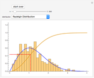
By "kernel-weighted", we mean that the data are weighted according to the Epanechnikov kernel 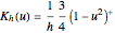 , where
  ,
,  is a design point, and
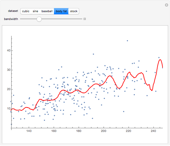
  is the "kernel bandwidth". The variable effectively controls the amount of nearby data that are permitted to influence the estimate of (and its derivatives) locally. There are a variety of techniques or heuristics available to choose . You can vary the size of the bandwidth. Smaller bandwidths reveal too many of the local features of the data, perhaps, and larger bandwidths oversmooth the data.
By solving a kernel-weighted least squares regression at each design point, we obtain an estimate of the value of and its first two derivatives at each design point. We then have all the information we need to fit a spline.
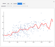
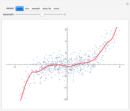
The "cubic" set of data is a simulated set formed by generating 600 realizations of with a standard normal distribution and then simulating 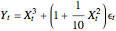 , where are independently simulated standard normal random variables.
The "sine" set of data is another simulated set, formed by first generating 600 realizations of with a uniform distribution over the interval  . We then obtain simulations of according to the rule
 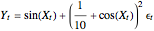 , where are independently simulated standard normal random variables.
The "baseball" data consists of performance data for all regular major league baseball players during the 1999 baseball season. We compute the overall proportion of hits to at-bats, and the proportion of hits to at-bats when there is a teammate in scoring position. The two proportions are obviously positively correlated, but the nonlinear regression model offers a potentially more useful fit than the usual linear regression model. These data were taken from John Rasp's website.
The "body fat" data were also taken from John Rasp's website. The data were taken from a sample of 252 men. The covariate  is the weight (in pounds) of the male subject, and the dependent variable
  is the body fat percentage (obtained through an underwater weighing procedure).
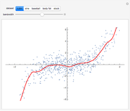
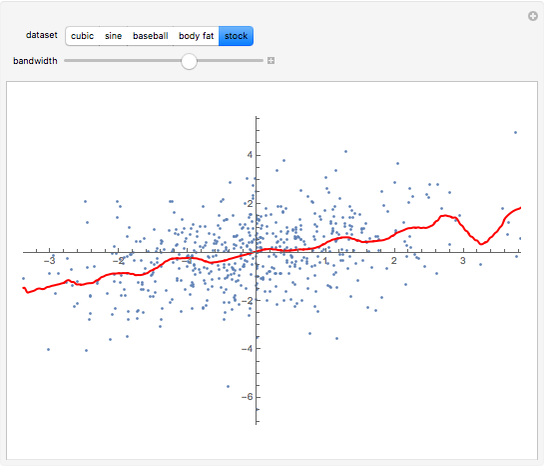
The "stock" data consists of U.S. equity returns ( variable) and French equity returns ( variable) for 1000 trading days in the late 1990s.
Permanent Citation
 Kernel Density Estimation
Jeff Hamrick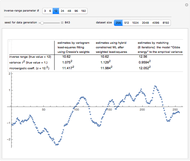 Estimating a Centered Matérn (1) Process: Three Alternatives to Maximum Likelihood via Conjugate Gradient Linear Solvers
Didier A. Girard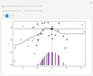 How Loess Works
Ian McLeod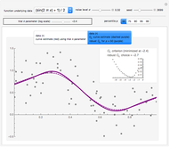 Nonparametric Curve Estimation by Smoothing Splines: Unbiased-Risk-Estimate Selector and its Robust Version via Randomized Choices
Didier A. Girard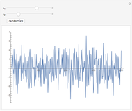 Auto-Regressive Simulation (Second-Order)
David von Seggern (University of Nevada)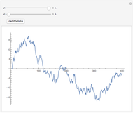 Autoregressive Moving-Average Simulation (First Order)
David von Seggern (University of Nevada)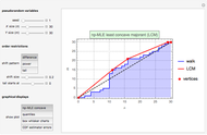 Estimating a Distribution Function Subject to a Stochastic Order Restriction
Michail Bozoudis and Vasileios Papachatzis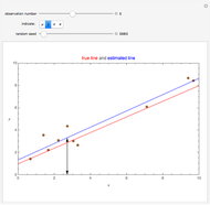 Mean, Fitted-Value, Error, and Residual in Simple Linear Regression
Ian McLeod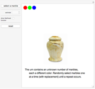 Maximum Likelihood Estimation
Marc Brodie (Wheeling Jesuit University)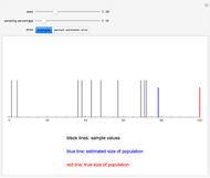 Estimating the Size of a Population
Heikki Ruskeepää
-
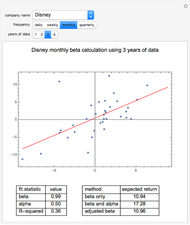 Expected Returns of the Dow Industrials, Beta Model
Jeff Hamrick -
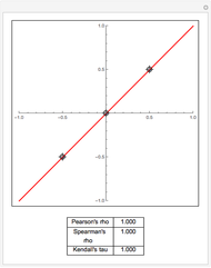 Exploring Measures of Association
Jeff Hamrick -
 Bootstrapping Credit Default Swap Data
Jeff Hamrick -
 Linear Dependence between Two Bernoulli Random Variables
Jeff Hamrick -
 Estimating the Local Mean Function
Jeff Hamrick -
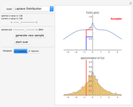 Acceptance/Rejection Sampling
Jeff Hamrick -
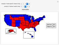 Simulating the 2008 U.S. Presidential Election
Jeff Hamrick -
 The Method of Inverse Transforms
Jeff Hamrick -
 The Perturbed Rat
Jeff Hamrick -
 Modeling Return Distributions
Jeff Hamrick -
 Pricing a European-Style Arithmetic Asian Option: Comparing Bootstrapping and Simulation Approaches
Jeff Hamrick -
 The Method of Common Random Numbers: An Example
Jeff Hamrick -
 The Envelope Theorem: Numerical Examples
Jeff Hamrick -
 Bootstrapping to Compute Value-at-Risk Standard Errors
Jeff Hamrick -
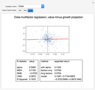 Expected Returns of the Dow Industrials, Fama-French Model
Jeff Hamrick -
Kernel Density Estimation
Jeff Hamrick -
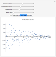 Simulating Asset Prices with a GARCH(1,1) Model
Jeff Hamrick