Forward and Inverse Kinematics for Two-Link Arm


Requires a Wolfram Notebook System
Interact on desktop, mobile and cloud with the free Wolfram Player or other Wolfram Language products.
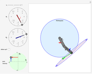
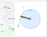
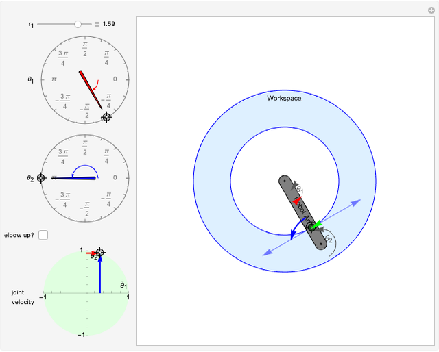
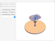
This Demonstration lets you control a two-link revolute-revolute robot arm either by setting the two joint angles (this is called forward kinematics) or by dragging a locator specifying the tip of the end effector (this is called inverse kinematics). Most locations in the workspace have two solutions to the inverse kinematics and can be selected with the "elbow up?" check box. The joint velocities are limited to magnitudes less than or equal to 1, represented by a green disc. Joint velocities map to a velocity of the end effector, drawn with a green locator (this is called forward velocity kinematics). Dragging the green locator maps to joint velocities (this is called inverse velocity kinematics). You can vary the relative link lengths under the constraint that  .
.
Contributed by: Aaron T. Becker and Lillian Lin (June 2016)
Open content licensed under CC BY-NC-SA
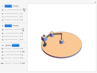
Snapshots


Details
A robot arm, or robot manipulator, is constructed from two types of joints, prismatic and revolute. A revolute joint rotates on a single plane along an axis centered at the joint, while a prismatic joint moves linearly, extending along a line. The transformation from joint angles to the location of the end effector is called forward kinematics and can be computed by a series of matrix multiplications.
Each joint transforms the coordinate frame from the previous joint. These coordinate transformations are multiplied together to determine the location of the end effector. The Denavit–Hartenberg convention represents the transformation due to the  joint as [1]:
 , where
  and
and  .
.
A sequence of matrices  are then multiplied together to give the location of the end effector.
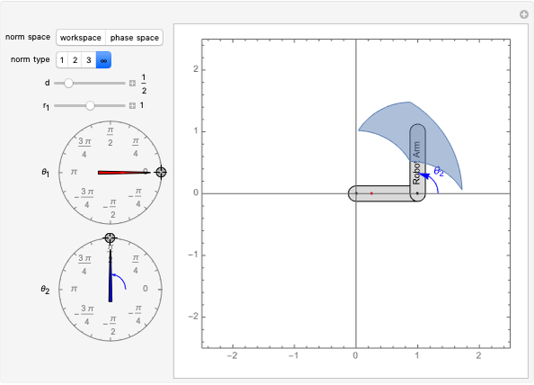
The transformation from the end effector location to joint angles is usually challenging because it often involves inverse trigonometric functions. Often there are multiple solutions, and the transformation is sometimes impossible (some end effectors are outside the workspace of the robot). Even for this simple two-link robot, these issues are present. The reachable workspace is drawn in blue. All locations outside of this region are impossible to reach. All locations on the boundary of this workspace have only one solution, but locations inside the blue region can be reached by two configurations, called the "elbow up" and "elbow down" configurations.
The transformation from joint velocities  to end effector velocities
  is called forward velocity kinematics. It can be computed by taking the derivative of the forward kinematics equations and multiplying this by the joint velocities. This gives the Jacobian, a function of the current robot configuration and is represented by
  , where
  is a vector of joint angles:
 .
.
If all joint velocities are within the unit ball  , then the end effector velocities are constrained to lie within an ellipse, drawn in pink in the figure. This ellipse is called the manipulability ellipse.
The inverse problem of determining what joint velocities  are required to generate a desired
  is inverse velocity kinematics. Inverse velocity kinematics is trivial if
  exists:
  , but when
  is singular this is not possible. In this Demonstration, singular configurations occur on the boundary of the workspace, where the manipulability ellipse loses a dimension and becomes a line. In this case, we solve for the required joint velocities by generating the Moore–Penrose pseudoinverse. This is calculated in Mathematica as PseudoInverse[J]·ξ= q'.
Reference
[1] M. W. Spong, S. Hutchinson, and M. Vidyasagar, Robot Modeling and Control, Hoboken, NJ: John Wiley and Sons, 2006.
Permanent Citation
 Denavit-Hartenberg Parameters for a Three-Link Robot
Aaron T. Becker and Mary Burbage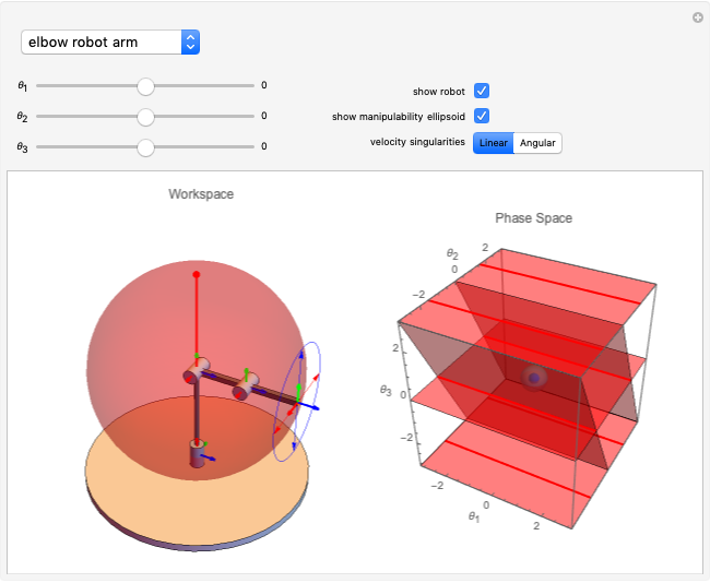 Robot Singularities in Three-Link Manipulators
Aaron T. Becker and Yitong Lu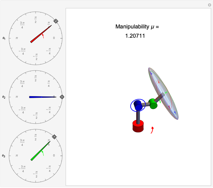 Manipulability Ellipsoid of a Robot Arm
Aaron T. Becker and Mary Burbage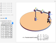 Common Robot Arm Configurations
Mohammad Sultan and Aaron T. Becker Probabilistic Roadmap Method for Robot Arm
Aaron T. Becker and Yitong Lu Probabilistic Roadmap Method with Seven-Link Articulated Robot
Aaron T. Becker and Yitong Lu Ensemble Control of Robots with Unicycle Kinematics
Aaron Becker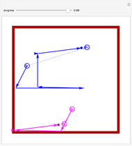 Moving Two Particles with Shared Control Inputs Using Wall Friction
Shiva Shahrokhi and Aaron T. Becker Forward and Inverse Kinematics of the SCARA Robot
Frederick Wu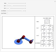 Forward Kinematics
Rob Lockhart
-
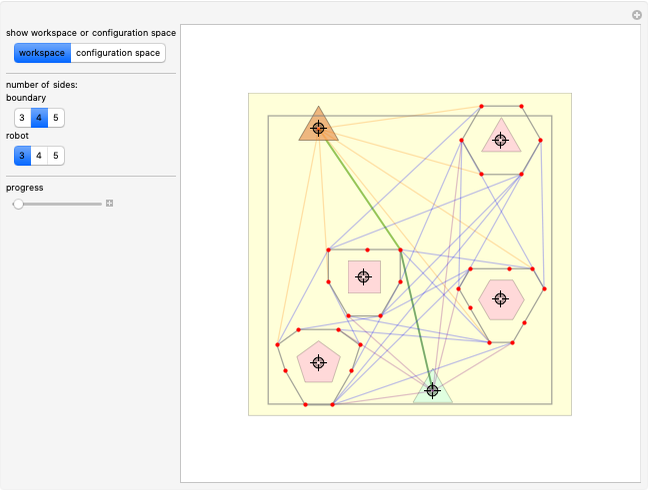
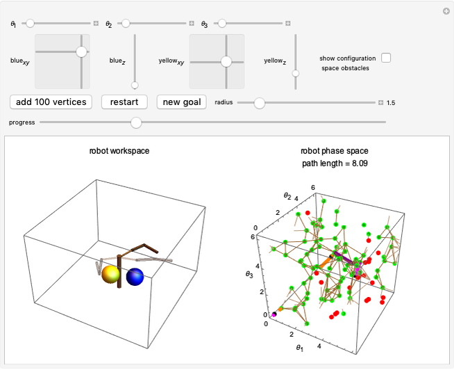
 Distance Norms in Robot Workspace and Phase Space
Aaron T. Becker -
 Forward and Inverse Kinematics for Two-Link Arm
Aaron T. Becker -
Manipulability Ellipsoid of a Robot Arm
Aaron T. Becker -
 Projected Area of a Cuboid
Aaron T. Becker -
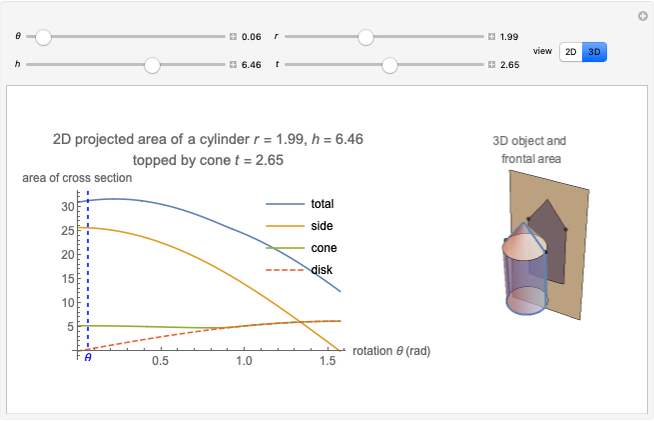 Projected Areas of Cylinder and Cone
Aaron T. Becker -
Robot Singularities in Three-Link Manipulators
Aaron T. Becker -
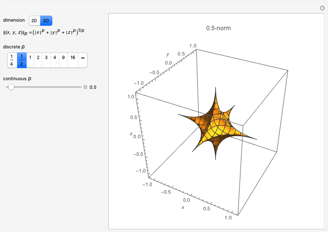 Unit Balls for Different p-Norms in 2D and 3D
Aaron T. Becker -
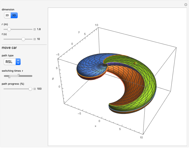 3D Reachability Set for a Dubins Car
Aaron T. Becker -
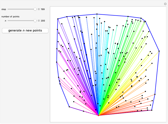 Graham Scan to Find the Convex Hull of a Set of Points in 2D
Aaron T. Becker -
 Motion Planning for Robot Path around Obstacles
Aaron T. Becker -
Probabilistic Roadmap Method with Seven-Link Articulated Robot
Aaron T. Becker -
 Probabilistic Roadmap Method in 3D
Aaron T. Becker -
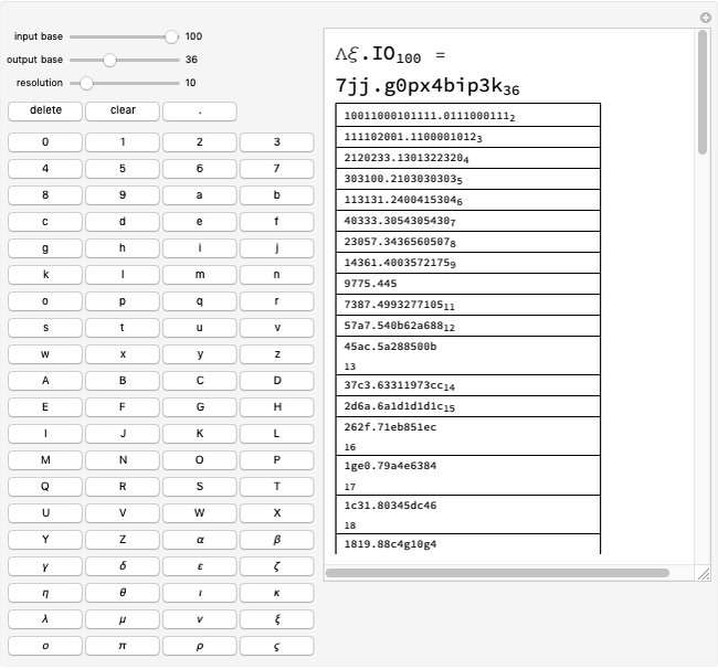 Base Conversions from Base 2 through 100 Using Radix Points
Aaron T. Becker -
Probabilistic Roadmap Method for Robot Arm
Aaron T. Becker -
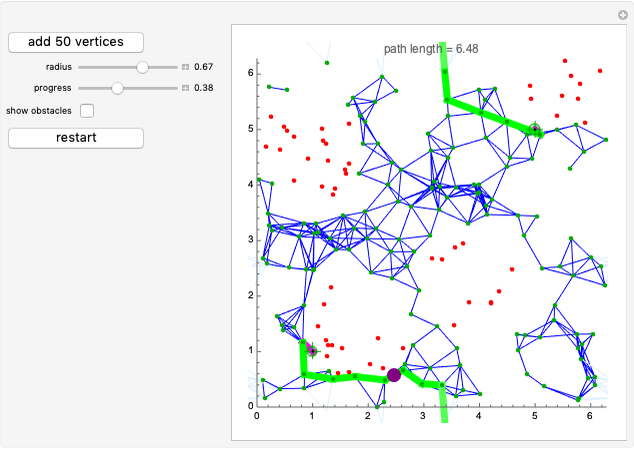 Probabilistic Roadmap Method
Aaron T. Becker -
 Robot Manipulator Workspaces
Aaron T. Becker -
 Reachable Set for a Drone
Aaron T. Becker -
 Smallest Circle Problem
Aaron T. Becker -
 Art Gallery Problem
Aaron T. Becker -
 Visibility Region of a Polygon
Aaron T. Becker