Isoperiodic Potentials via Series Expansion


Requires a Wolfram Notebook System
Interact on desktop, mobile and cloud with the free Wolfram Player or other Wolfram Language products.
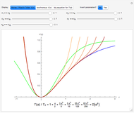
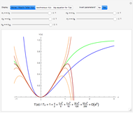
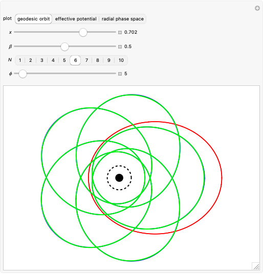
In a one-dimensional oscillation obeying conservation of energy, the potential function determines the period of motion  as a function of dimensionless energy
  . However, the period function
  only uniquely determines the potential
  in the case of parity symmetry, where
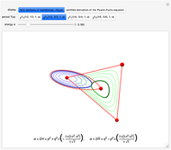
  . In all other cases, it is possible to construct an uncountable infinity of potentials with the same period . Regardless of symmetry, we call any two potentials isoperiodic if they have the same period function [1]. Careful examination of inverse functions leads to a precise definition of isoperiodic potentials using power series expansion [2]. As in [3], we use a phase-space technique to write as a function of the potential expansion coefficients around a stable minima. The general form of leads to a set of linear constraints between the expansion coefficients of isoperiodic potentials (see Details).

Contributed by: Brad Klee (April 2017)
Open content licensed under CC BY-NC-SA
Snapshots


Details
For details of published calculations, see [1, 2]. Our approach follows [3]. Starting with a Hamiltonian
 ,
,
we transform to the polar coordinates of phase space
 ,
,
where  . The preceding algorithm approximately solves this implicit equation by series inversion, producing a truncated sum
 .
.
The corresponding approximate period is then calculated using
 .
.
Analyzing the general period function  first reported in [4], we prove that every power of the Hamiltonian energy
  attaches to a function of the potential expansion coefficients
  with a pair
  that does not occur in the coefficient of any
  with
with  . This fact allows order-by-order construction of isoperiodic potentials as series expansions around a stable minima.
The isoperiodic constraint between two distinct potentials with expansion coefficients  and
and  is
is
 .
.
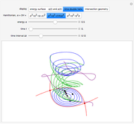
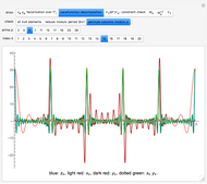
Fixing the values and applying the isoperiodic constraint to the yet leaves one continuous degree of freedom in every coefficient  . These continuous degrees of freedom are controlled by sliders in this Demonstration, which directly enables you to calculate a range of isoperiodic potentials. Methods used here have also contributed to award-winning posts on Wolfram Community [5, 6].
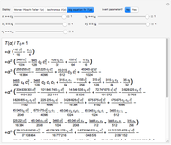
By direct evaluation of the period function for the expansion coefficients of the Morse potential and the Pöschl–Teller potential, it is possible to prove approximate isoperiodicity order-by-order, as in the commented code at the end of the initialization section. Comparing coefficients, we expect direct evaluation of both period integrals to yield
 .
.
References
[1] M. Asorey, J. F. Cariñena, G. Marmo and A. Perelomov, "Isoperiodic Classical Systems and Their Quantum Counterparts," Annals of Physics, 322(6), 2007 pp. 1444–1465. doi:10.1016/j.aop.2006.07.003.
[2] E. T. Osypowski and M. G. Olsson, "Isynchronous Motion in Classical Mechanics," American Journal of Physics, 55(8), 1987 pp. 720–725. doi:10.1119/1.15063.
[3] B. Klee, "Plane Pendulum and Beyond by Phase Space Geometry." arxiv.org/abs/1605.09102.
[4] The On-Line Encyclopedia of Integer Sequences. (Apr 4, 2017) oeis.org/A276816.
[5] B. Klee, "A Period Function for Anharmonic Oscillations" from Wolfram Community—A Wolfram Web Resource. (Apr 4, 2017) community.wolfram.com/groups/-/m/t/984488.
[6] B. Klee, "Plotting the Contours of Deformed Hyperspheres" from Wolfram Community—A Wolfram Web Resource. (Apr 4, 2017) community.wolfram.com/groups/-/m/t/1023763.
Permanent Citation
 Modeling a Simple Roller Coaster
Erik Mahieu Boole Differential Equation with Continued Fractions
Andreas Lauschke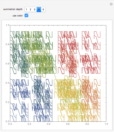 Schoenberg Plane-Filling Curve
Robert Dickau Motion on a Surface
Tomas Kalvoda Motion of Exploding Projectile
Hannah Rudin Superposition of Transverse Simple Harmonic Waves
Cássio Pigozzo Chebyshev Walking Machine
Erik Mahieu Designs from Mechanical Linkages
Erik Mahieu Offset Slider-Crank Mechanism
Erik Mahieu Trace Curves Produced by Crank-Slider Mechanism
Gábor Erdös
-
 Deriving Hypergeometric Picard-Fuchs Equations
Brad Klee -
 Discrete and Continuous Quartic Anharmonic Oscillation
Brad Klee -
 Edwards's Solution of Pendulum Oscillation
Brad Klee -
 Weierstrass Solution of Cubic Anharmonic Oscillation
Brad Klee -
 Molien Series for a Few Double Groups
Brad Klee -
 Factoring the Even Trigonometric Polynomials of A269254
Brad Klee -
 Multipole Expansions of Electric Fields
Brad Klee -
 Series Approximation for the Schwarz D Surface
Brad Klee -
 Isoperiodic Potentials via Series Expansion
Brad Klee -
 Estimating Planetary Perihelion Precession
Brad Klee -
 Exact and Approximate Relativistic Corrections to the Orbital Precession of Mercury
Brad Klee -
 Drawing Paths on the Sierpinski Carpet
Brad Klee -
 Transformation of Icosahedral Solids in Z15
Brad Klee -
 Approximating the Jacobian Elliptic Functions
Brad Klee -
 Stereographic Projection of Some Double Groups
Brad Klee -
 Quantum Angular Momentum Matrices
Brad Klee -
 Flowsnake Q-Function
Brad Klee -
 Limit-Periodic Tilings
Brad Klee -
 Projections of Polyhedra Stellation
Brad Klee -
 Tensor Equation of a Plane
Brad Klee