The Difference between European Option Prices in the Black-Scholes and NIG Models Computed with the DFT


Requires a Wolfram Notebook System
Interact on desktop, mobile and cloud with the free Wolfram Player or other Wolfram Language products.
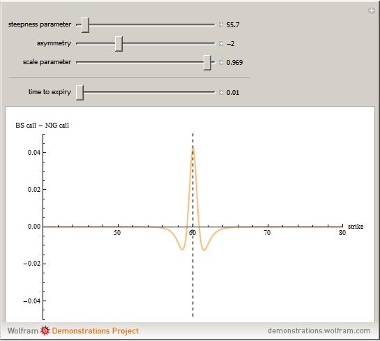
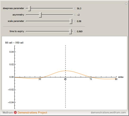
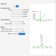
This Demonstration shows the difference between the price of a European call option on stock (no dividend is paid and the interest rate is 0) in the Black–Scholes model and the model (due to Barndorff–Nielson) based on a centered exponential Normal Inverse Gaussian (NIG) Lévy process, as a function of the strike price. There are three model parameters that control the NIG process: steepness, asymmetry, and scale (the fourth parameter, location, is set to 0). The other control parameter is the time to expiry of the option.
[more]
Contributed by: Andrzej Kozlowski (March 2011)
Open content licensed under CC BY-NC-SA
Snapshots

Details
The NIG process has been shown by several empirical studies to model option prices more accurately than the Black–Scholes model. Unlike the Black–Scholes model, there is no unique non-arbitrage price in the NIG model (and in other incomplete models, e.g. those involving jumps or stochastic volatility), so the price has to be chosen using economic considerations. We use the price given by replacing the real world measure by the equivalent martingale measure defined by means of the Esscher transform (see [2]). The prices for both models are computed for a range of strike prices using the discrete Fourier transform (DFT) following the method described in [1] and generalized in [3]. The method of computing NIG option prices used in this Demonstration is due to Gerber and Shiu [1]. A detailed study of option pricing with Lévy processes, of which the NIG process is an example, can be found in [2].
[1] P. Carr and D. B. Madan, "Option Valuation Using the Fast Fourier Transform," The Journal of Computational Finance, 2(4), 1999.
[2] H. U. Gerber and E. S. W. Shiu, "Option Pricing by Esscher Transforms," Transactions of the Society of Actuaries, 46, 1999 pp. 99–191.
[3] S. Raible, Lévy Processes in Finance: Theory, Numerics, and Empirical Facts, PhD thesis, University of Freiburg, 2000.
 Option Prices under the Fractional Black-Scholes Model
Andrzej Kozlowski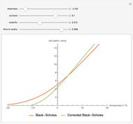 The Black-Scholes European Call Option Formula Corrected Using the Gram-Charlier Expansion
Andrzej Kozlowski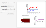 Hedging the Black-Scholes Call Option
Andrzej Kozlowski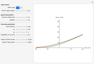 Option Prices in the Kou Jump Diffusion Model
Andrzej Kozlowski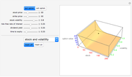 Exploring the Black-Scholes Formula
Andrzej Kozlowski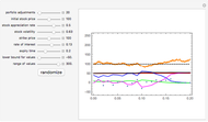 Hedging the European Put Option
Andrzej Kozlowski Standard American and European Options
Andrzej Kozlowski The Price of a Call Option on Electrical Power
Andrzej Kozlowski Pricing a Bermudan Option with the Longstaff-Schwartz Monte Carlo Method
Andrzej Kozlowski The Russian Option: Reduced Regret
Andrzej Kozlowski
-
The Black-Scholes European Call Option Formula Corrected Using the Gram-Charlier Expansion
Andrzej Kozlowski -
Option Prices in the Kou Jump Diffusion Model
Andrzej Kozlowski -
 The Polar and Bipolar of a Convex Polytope
Andrzej Kozlowski -
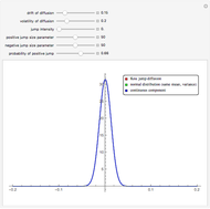
 Two Jump Diffusion Processes
Andrzej Kozlowski -
 The Vieta Mapping for the Coxeter Group A_2
Andrzej Kozlowski -
 The Bifurcation Set of the Space of Smooth Real Functions
Andrzej Kozlowski -
 The Swallowtail Singularity
Andrzej Kozlowski -
 Singularities of an Ellipsoidal Wave Front
Andrzej Kozlowski -
 Nonuniqueness of Option Pricing Under the Meixner Model
Andrzej Kozlowski -
 Coin Machine
Andrzej Kozlowski -
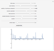 A Mean-Reverting Jump Diffusion Process
Andrzej Kozlowski -
Standard American and European Options
Andrzej Kozlowski -
 Density of the Kou Jump Diffusion Process
Andrzej Kozlowski -
 The Meixner Process
Andrzej Kozlowski -
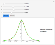 Fitting the Meixner Distribution to S&P 500 Returns
Andrzej Kozlowski -
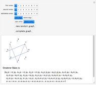 Simple Graphs and Their Binomial Edge Ideals
Andrzej Kozlowski -
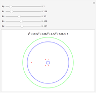 The Eneström-Kakeya Bounds for Roots of a Polynomial with Positive Coefficients
Andrzej Kozlowski -
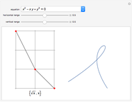 Newton Polygon and Branching of Algebraic Curves
Andrzej Kozlowski -
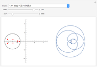 Counting the Number of Roots of Transcendental Functions in Bounded Regions Using Winding Numbers
Andrzej Kozlowski -
 The Space of Inner Products
Andrzej Kozlowski