Chaotic Quantum Motion of Two Particles in a 3D Harmonic Oscillator Potential


Requires a Wolfram Notebook System
Interact on desktop, mobile and cloud with the free Wolfram Player or other Wolfram Language products.
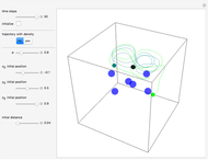
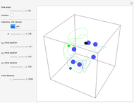
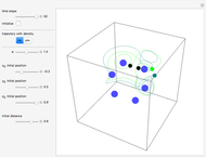
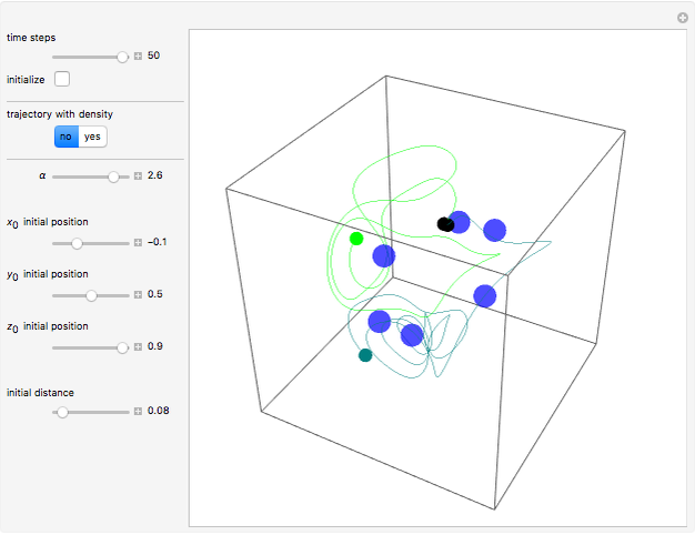
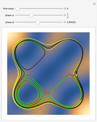
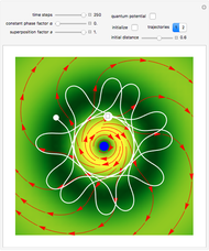
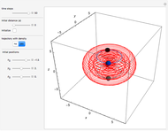
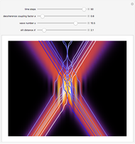
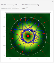
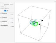
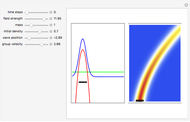
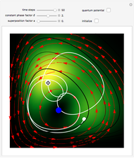
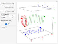
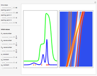
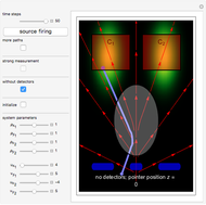
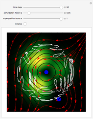
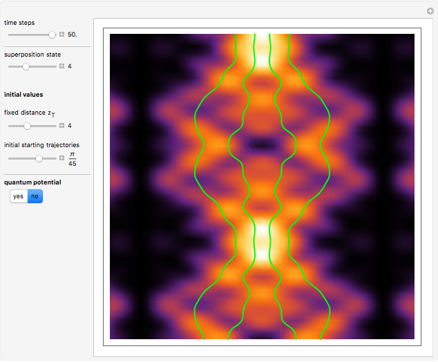
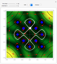
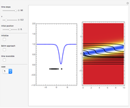
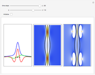
A system with three degrees of freedom, consisting of a superposition of three coherent stationary eigenfunctions with commensurate energy eigenvalues and a constant relative phase, can exhibit chaotic motion in the de Broglie–Bohm formulation of quantum mechanics (see Quantum Motion of Two Particles in a 3D Trigonometric Pöschl–Teller Potential). We consider here an analog using a three-dimensional harmonic-oscillator potential. In this case, the velocities of the particles are autonomous, with a complex, chaotic trajectory structure. Two particles are placed randomly, separated by an initial distance  , on the boundary of the harmonic potential.
Contributed by: Klaus von Bloh (July 2015)
Open content licensed under CC BY-NC-SA
Snapshots


Details
Associated Hermite polynomials arise as the solution of the Schrödinger equation:
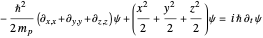 ,
with
,
with  ,
,  , and so on. A degenerate, unnormalized, complex-valued wavefunction
  for the three-dimensional case can be given by:
 ,
,
where  ,
,  ,
,  are eigenfunctions, and
  are permuted eigenenergies of the corresponding stationary one-dimensional Schrödinger equation with
  . The eigenfunctions are defined by
 ,
,
where  ,
,  ,
,  are Hermite polynomials. The parameter
  is a constant phase shift. The eigenvalues' numbers
  depend on the three quantum numbers
  .
.
In this Demonstration, the wavefunction  is defined by:
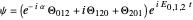 .
.
In this case, the square of the Schrödinger wavefunction  , where
  is its complex conjugate, is not time dependent:
 .
.
The velocity field  is calculated from the gradient of the phase from the total wavefunction in the eikonal form (often called polar form)
  . The time-dependent phase function
  from the total wavefunction
  is:
is:
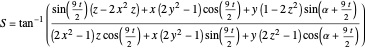 .
.
The corresponding velocity field becomes time independent (autonomous) because of the time-independent gradient of the phase function.
In the program, if PlotPoints, AccuracyGoal, PrecisionGoal, MaxSteps, and MaxIterations are enabled, increasing them will give more accurate results.
References
[1] "Bohmian-Mechanics.net." (Jul 30, 2015) www.bohmian-mechanics.net/index.html.
[2] S. Goldstein. "Bohmian Mechanics." The Stanford Encyclopedia of Philosophy. (Jul 30, 2015)plato.stanford.edu/entries/qm-bohm.
Permanent Citation
 Simple Chaotic Motion of Quantum Particles According to the Causal Interpretation of Quantum Theory
Klaus von Bloh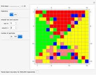 Mixing of Quantum Particles Influenced by Nodal Points in the Causal Interpretation
Klaus von Bloh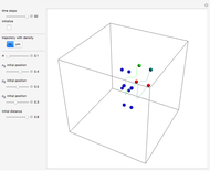 Periodic Quantum Motion of Two Particles in a 3D Harmonic Oscillator Potential
Klaus von Bloh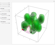 Bohm Trajectories for a Particle in an Infinite 3D Box
Klaus von Bloh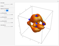 Quantum Motion of Two Particles in a 3D Trigonometric Pöschl-Teller Potential
Klaus von Bloh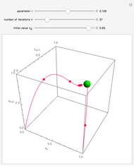 3D Poincaré Plot of the Logistic Map
Narken Aimambet 2D and 3D Packard-Takens Autocorrelation Plots of Sinusoidal Functions
Mark D. Normand and Micha Peleg Time Evolution of a Quantum Free Particle in 2D
Porscha McRobbie and Eitan Geva Addition of Angular Momenta in Quantum Mechanics
S. M. Blinder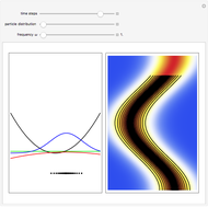 Causal Interpretation of the Quantum Harmonic Oscillator
Klaus von Bloh
-
 Bohm Trajectories for the Two-Dimensional Coulomb Potential
Klaus von Bloh -
 Bohm Trajectories in an LCAO Approximation for the Hydrogen Molecule H_2
Klaus von Bloh -
 Decoherence and Trajectories Implied by a Modified Schrodinger Equation
Klaus von Bloh -
 Bohm Trajectories for a Particle in a Two-Dimensional Circular Billiard
Klaus von Bloh -
 From Bohm to Classical Trajectories in a Hydrogen Atom
Klaus von Bloh -
 Continuous Transition between Quantum and Classical Behavior for a Harmonic Oscillator
Klaus von Bloh -
 Continuous Transition between Classical and Bohm Quantum Pictures for Young's Interference Experiment
Klaus von Bloh -
 Bohm Trajectories for Quantum Particles in a Uniform Gravitational Field
Klaus von Bloh -
 Bohm Trajectories for a Particle in a Two-Dimensional Calogero-Moser Potential
Klaus von Bloh -
 Nonlocality in the de Broglie-Bohm Interpretation of Quantum Mechanics
Klaus von Bloh -
 Three-Soliton Collision in the Trajectory Approach
Klaus von Bloh -
 The Which-Way Experiment and the Conditional Wavefunction
Klaus von Bloh -
 Chaotic Quantum Motion of Two Particles in a 3D Harmonic Oscillator Potential
Klaus von Bloh -
 Perturbation Theory in the de Broglie-Bohm Interpretation of Quantum Mechanics
Klaus von Bloh -
Periodic Quantum Motion of Two Particles in a 3D Harmonic Oscillator Potential
Klaus von Bloh -
Quantum Motion of Two Particles in a 3D Trigonometric Pöschl-Teller Potential
Klaus von Bloh -
 The Talbot Carpet in the Causal Interpretation of Quantum Mechanics
Klaus von Bloh -
 Bohmian Quantum Trajectories for Coherent States of the Pöschl-Teller Potential
Klaus von Bloh -
 Gray and Dark Solitons in the de Broglie and Bohm Approaches
Klaus von Bloh -
 A Breather Solution in the Causal Interpretation of Quantum Mechanics
Klaus von Bloh