Radioactive Decay in the Causal Interpretation of Quantum Theory

Requires a Wolfram Notebook System
Interact on desktop, mobile and cloud with the free Wolfram Player or other Wolfram Language products.
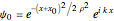
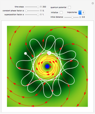
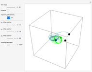
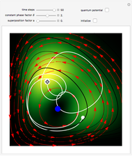
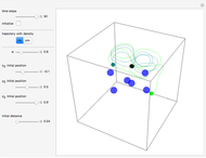
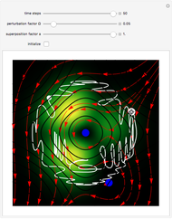
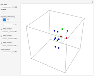
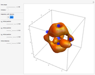
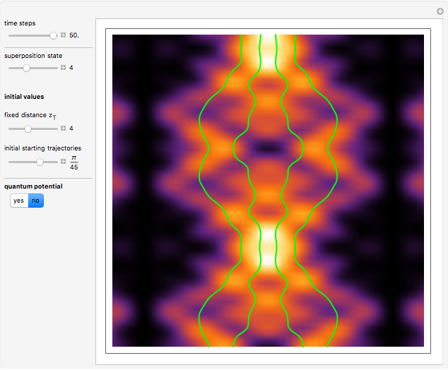
According to classical physics, a particle can never overcome a potential greater than its kinetic energy; this is not the case in quantum theory. For unstable isotopes there is a finite probability for a quantum particle (an  particle) to tunnel through the potential barrier in a nucleus. Such isotopes are called radioactive isotopes. The behavior of such isotopes can be described by a square wave packet that is a solution of the Schrödinger equation with the potential term
  . The time evolution leads to a wave packet that bounces back and forth. Each time it strikes the potential barrier a part of the packet tunnels through and there is a chance for some transmission. In orthodox quantum theory it is impossible to predict the decay of a single isotope. A statistical conclusion can be made only for an ensemble of isotopes (e.g., half-life period).


Contributed by: Klaus von Bloh (December 2008)
Based on a program by: Enrique Zeleny and Paul Nylander
Open content licensed under CC BY-NC-SA
Snapshots


Details
The guidance equation for the particle velocity is  , which is calculated from the gradient of the phase from the total wavefunction in the eikonal form
  . The quantum potential
  is given by
  . The effective potential is the sum of quantum potential and nuclear potential that leads to the time-dependent quantum force:
  . The numerical methods to calculate the velocity and the quantum potential from a discrete function are, in general, not very stable, but the applied interpolation functions lead to an accurate approximation of the physical event; due to the numerical errors produced by the limited mesh of 120 mesh points, the velocity term must be adjusted (here using 41/100 instead of 0.5).
References
C. Dewdney and B. J. Hiley, "A Quantum Potential Description of One-Dimensional Time-Dependent Scattering from Square Barriers and Square Wells," Found. Phys. 12(1), 1982 pp. 27–48.
J. Caulfield, "What Determines Alpha Decay?," Portsmouth Polytechnic (England), student research project, unpublished, 1991.
A. Goldberg, H. Schey, and J. L. Schwartz, "Computer-Generated Motion Pictures of One-Dimensional Quantum Mechanical Transmission and Reflection Phenomena," Am. J. Phys., 35(3), 1967 pp. 177–186.
Permanent Citation
 Causal Interpretation of the Free Quantum Particle
Klaus von Bloh Soliton Trajectories of the Modified Korteweg-de Vries Equation (mKdV)
Klaus von Bloh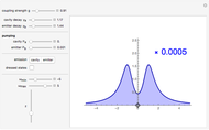 Cavity Quantum Electrodynamics with Bosons: Emission Spectra in the Strong and Weak Coupling Regimes
Fabrice P. Laussy and Elena del Valle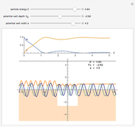 Scattering by a Square-Well Potential
M. Hanson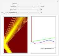 Time-Dependent Scattering in the Causal Interpretation of Quantum Theory
Klaus von Bloh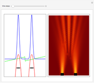 Causal Interpretation of the Double-Slit Experiment in Quantum Theory
Klaus von Bloh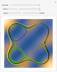 Simple Chaotic Motion of Quantum Particles According to the Causal Interpretation of Quantum Theory
Klaus von Bloh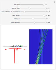 The Causal Interpretation of Quantum Tunneling through a Square Barrier and Well
Klaus von Bloh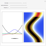 Causal Interpretation of the Quantum Harmonic Oscillator
Klaus von Bloh Entanglement between a Two-Level System and a Quantum Harmonic Oscillator
Kwan-yuet Ho
-
 Bohm Trajectories for the Two-Dimensional Coulomb Potential
Klaus von Bloh -
 Bohm Trajectories in an LCAO Approximation for the Hydrogen Molecule H_2
Klaus von Bloh -
 Decoherence and Trajectories Implied by a Modified Schrodinger Equation
Klaus von Bloh -
 Bohm Trajectories for a Particle in a Two-Dimensional Circular Billiard
Klaus von Bloh -
 From Bohm to Classical Trajectories in a Hydrogen Atom
Klaus von Bloh -
 Continuous Transition between Quantum and Classical Behavior for a Harmonic Oscillator
Klaus von Bloh -
 Continuous Transition between Classical and Bohm Quantum Pictures for Young's Interference Experiment
Klaus von Bloh -
 Bohm Trajectories for Quantum Particles in a Uniform Gravitational Field
Klaus von Bloh -
 Bohm Trajectories for a Particle in a Two-Dimensional Calogero-Moser Potential
Klaus von Bloh -
 Nonlocality in the de Broglie-Bohm Interpretation of Quantum Mechanics
Klaus von Bloh -
 Three-Soliton Collision in the Trajectory Approach
Klaus von Bloh -
 The Which-Way Experiment and the Conditional Wavefunction
Klaus von Bloh -
 Chaotic Quantum Motion of Two Particles in a 3D Harmonic Oscillator Potential
Klaus von Bloh -
 Perturbation Theory in the de Broglie-Bohm Interpretation of Quantum Mechanics
Klaus von Bloh -
 Periodic Quantum Motion of Two Particles in a 3D Harmonic Oscillator Potential
Klaus von Bloh -
 Quantum Motion of Two Particles in a 3D Trigonometric Pöschl-Teller Potential
Klaus von Bloh -
 The Talbot Carpet in the Causal Interpretation of Quantum Mechanics
Klaus von Bloh -
 Bohmian Quantum Trajectories for Coherent States of the Pöschl-Teller Potential
Klaus von Bloh -
 Gray and Dark Solitons in the de Broglie and Bohm Approaches
Klaus von Bloh -
 A Breather Solution in the Causal Interpretation of Quantum Mechanics
Klaus von Bloh