Uncertainties in Isothermal Microbial Growth


Requires a Wolfram Notebook System
Interact on desktop, mobile and cloud with the free Wolfram Player or other Wolfram Language products.
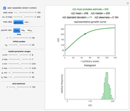
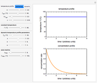
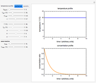
This Demonstration estimates a theoretical spread in the size of a microbial population in a closed habitat at a constant temperature at a given time. It is based on the assumption that the growth curve follows the shifted logistic model. Hence the growth ratio, linear or logarithmic, is determined by three parameters: the approximate asymptotic value  , a measure of the growth curve's steepness at the exponential phase
  , and a marker of the inflection point
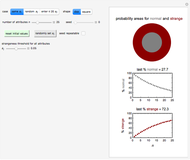
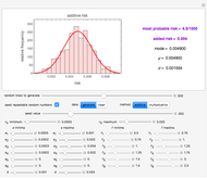
  . The three parameters are entered as the lower and upper limits of their plausible ranges. Monte Carlo simulations generate numerous hypothetical growth curves with random parameter values within the chosen ranges. The Demonstration displays a representative growth curve for the chosen parameter settings and the corresponding histogram and calculates the most probable population size for the chosen time along with some statistical characteristics of the generated data.
Contributed by: Mark D. Normand and Micha Peleg (December 2011)
Open content licensed under CC BY-NC-SA
Snapshots


Details
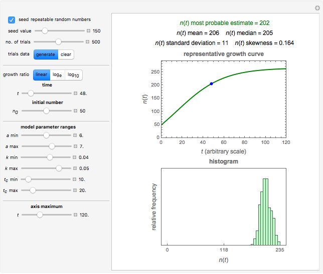
Snapshot 1: growth curve of 50 cells after 48 time units and corresponding histogram of the generated numbers calculated using the linear growth ratio
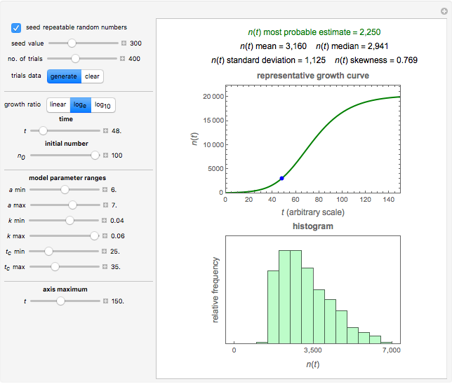
Snapshot 2: growth curve of 100 cells after 48 time units and corresponding histogram of the generated numbers calculated using the natural logarithmic growth ratio
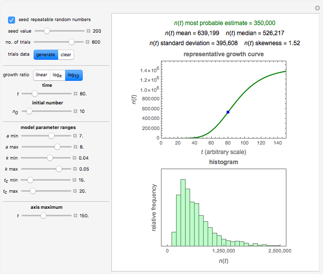
Snapshot 3: growth curve of 10 cells after 80 time units and corresponding histogram of the generated numbers calculated using the base 10 logarithmic growth ratio
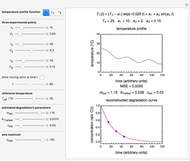
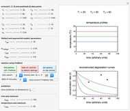
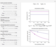
The isothermal growth curve of a microorganism is a plot of its population size (usually expressed as a count) versus time. When the growth takes place in a closed habitat and at a constant temperature, the curve is typically sigmoid initially and consists of three regions representing a "lag phase", an "exponential growth phase", and a "stationary phase". However, the latter cannot last indefinitely and eventually ends up in the onset of mortality. The sigmoid part of the growth curve can be described by a variety of interchangeable growth models, the shifted logistic model among them [1]. For mild, moderate, and intensive growth this model can be written as 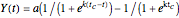 . For mild growth,
  might be the linear growth ratio
  , for moderate growth the natural logarithmic ratio
  , and for intensive growth, where the population rises by several orders of magnitude,
  . In all three cases,
  is the temporary number of cells after time
  and
and  their initial number. This implies that the growth curve itself in the three cases will be expressed as
  ,
, 
 , or
, or  , respectively.
According to this model, the growth parameters are (dimensionless), approximately the asymptotic growth ratio's level at the stationary phase, (time units reciprocal), a measure of the growth curve's steepness at its inflection point (the actual slope is  ), and
  (time units), a marker of the inflection point.
Since foods' composition and physical properties can and frequently do vary, there is always a degree of uncertainty concerning the magnitude of experimentally determined microbial growth parameters, and consequently in the predicted population size.
In this Demonstration you can enter the time , the plausible lower and upper bounds of the shifted logistic model's growth parameters,  ,
,  ,
,  ,
,  ,
,  , and
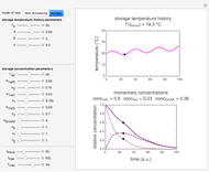
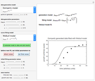
, and  with sliders, and also choose the number of Monte Carlo trials. Clicking the "seed repeatable random numbers" checkbox lets you reproduce the random simulation from the same seed value, also entered with a slider. The program then generates the chosen number of trials with random combinations of the growth parameters, assumed to be uniformly distributed within their respective ranges ("maximum ignorance") and calculates the corresponding growth curve using the shifted logistic model's equation with the chosen definition of the growth ratio (linear, natural logarithmic, or base 10 logarithmic) entered with a setter. The program plots a representative growth curve for the chosen parameters on which the slider-entered time is shown as a moving blue dot, and below it the histogram of the generated s for the entered settings. The most probable estimate of is the mean value of the histogram's bin having the largest number of entries. It is displayed accompanied by the generated counts' mean, median, standard deviation, and skewness. In order to produce new random trial data with exactly the same parameter settings, first click the "clear" and then the "generate" buttons.
Not all possible control settings produce realistic survival curves when the arbitrary time units are replaced by hours or days. The initial number's allowed range is 1 to 100. For larger numbers, multiply the results rendered by the Demonstration by the appropriate factor.
References
[1] M. Peleg, Advanced Quantitative Microbiology for Foods and Biosystems: Models for Predicting Growth and Inactivation, Boca Raton, FL: CRC Press, 2006.
[2] M. A. J. S. von Boekel, Kinetic Modeling of Reactions in Foods, Boca Raton: CRC Press, 2008.
[3] M. Peleg and M. G. Corradini, "Microbial Growth Curves — What the Models Tell Us and What They Cannot," CRC Critical Reviews in Food Science, 51, 2011 pp. 917–945.
[4] S. Smith-Simpson, M. G. Corradini, M. D. Normand, M. Peleg, and D. W. Schaffner, "Estimating Microbial Growth Parameters from Non-Isothermal Data: A Case Study with Clostridium perfringens," International Journal of Food Microbiology, 118, 2007 pp. 294–303.
[5] M. G. Corradini, A. Amézquita, M. D. Normand, and M. Peleg, "Modeling and Predicting Non-isothermal Microbial Growth Using General Purpose Software," International Journal of Food Microbiology, 106, 2006 pp. 223–328.
Permanent Citation
 Extending the Square Root Growth Rate Model to Lethal Low Temperatures
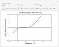
Mark D. Normand and Micha Peleg Model of Microbial Nutrient Uptake
Elena Beltrán-Heredia Lag Time in Microbial Growth
Mark D. Normand and Micha Peleg Extracting Microbial Inactivation Parameters from Final Isothermal Survival Ratios
Mark D. Normand and Micha Peleg Square Root Model for Rates of Microbial Growth or Inactivation
Mark D. Normand and Micha Peleg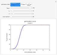 Isothermal Germination of Seeds and Microbial Spores
Mark D. Normand and Micha Peleg Injury in Microbial Inactivation
Mark D. Normand and Micha Peleg Stochastic Model of Microbial Injury and Mortality
Mark D. Normand , Maria G. Corradini, and Micha Peleg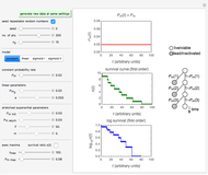 Probabilistic Model for Microbial Mortality
Mark D. Normand and Micha Peleg Degrees of Microbial Injury and Survival
Mark D. Normand and Micha Peleg
-
 Ratkowski's Square Root Growth Rate Model for High Temperatures
Micha Peleg -
 Gordon-Taylor and Fox Equations for Glass Transition Temperature
Micha Peleg -
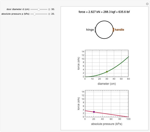 Force to Overcome Vacuum Pull
Micha Peleg -
Extending the Square Root Growth Rate Model to Lethal Low Temperatures
Micha Peleg -
 Probability of Being Strange According to Paulos
Micha Peleg -
 Successive Three-Point Method for Weibullian Chemical Degradation
Micha Peleg -
 Estimating Cohesion and Tensile Strength of Compacted Powders
Micha Peleg -
 Three-Endpoints Method for Isothermal Weibullian Chemical Degradation
Micha Peleg -
 Vitamin C Loss in Foods During Heat Processing and Storage
Micha Peleg -
 Parameterizing Temperature-Viscosity Relations
Micha Peleg -
 Laplace Distribution in Fluctuating Stock Index Records
Micha Peleg -
 Weibullian Chemical Degradation
Micha Peleg -
 Simulating Ascorbic Acid Degradation
Micha Peleg -
 Additive and Multiplicative Risks
Micha Peleg -
 Endpoints Method for Predicting Chemical Degradation in Frozen Foods
Micha Peleg -
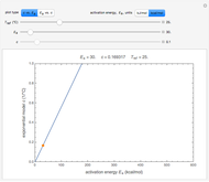 Exponential Model for Arrhenius Activation Energy
Micha Peleg -
 Prediction of Isothermal Degradation by the Endpoints Method
Micha Peleg -
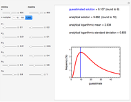 Risk Guesstimation from Factor Ranges
Micha Peleg -
 Volatiles Formation Kinetics in Stored Fish
Micha Peleg -
 Comparison of Six Sigmoid Growth Curve Models
Micha Peleg