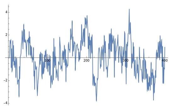
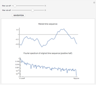
Auto-Regressive Simulation (Second-Order)


Requires a Wolfram Notebook System
Interact on desktop, mobile and cloud with the free Wolfram Player or other Wolfram Language products.
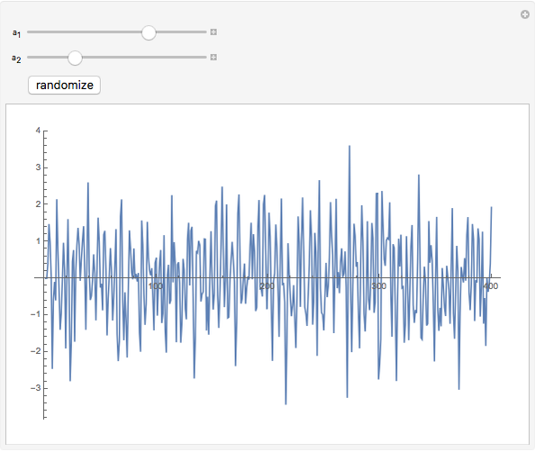
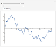
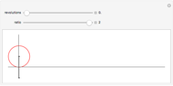
This Demonstration shows realizations of a second-order auto-regressive (AR) process  , using the random variable
  drawn from a normal density with mean zero and variance unity. It is governed by the equation:


Contributed by: David von Seggern (University of Nevada) (March 2011)
Open content licensed under CC BY-NC-SA
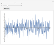
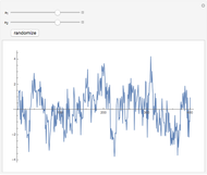
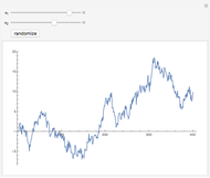
Snapshots


Details
The Demonstration is set such that the same random series of points is used no matter how the constants  and
and  are varied. However, when the "randomize" button is pressed, a new random series will be generated and used. Keeping the random series identical allows the user to see exactly the effects on the AR series of changes in the two constants. If the constants , do not meet the stationarity conditions, the series will diverge. The Demonstration is for a second-order process only. Additional AR terms would enable somewhat more complex series to be generated, but the differences from second-order processes would be difficult to ascertain.
For a detailed description of an AR process, see, for instance, G. M. Jenkins and D. G. Watts, Spectral Analysis and Its Applications, San Francisco: Holden-Day, 1968 or G. Box, G. M. Jenkins, and G. Reinsel, Time Series Analysis: Forecasting and Control, 3rd ed., Englewood Cliffs, NJ: Prentice-Hall, 1994.
Permanent Citation
 Autoregressive Moving-Average Simulation (First Order)
David von Seggern (University of Nevada) Simulating the Poisson Process
Heikki Ruskeepää Autoregressive Moving-Average Generator
Matus Baniar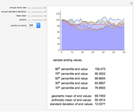 Mean-Reverting Random Walks
Jason Cawley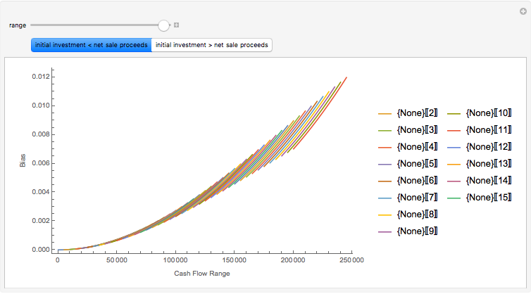 Simulating the IRR
Roger J. Brown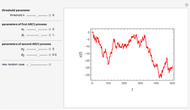 Two-Regime Threshold Autoregressive Model Simulation
Jozef Barunik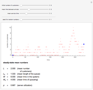 Simulating the M/M/1 Queue
Heikki Ruskeepää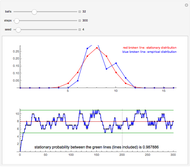 Simulating the Bernoulli-Laplace Model of Diffusion
Heikki Ruskeepää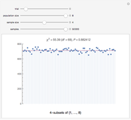 Goodness of Fit for Random Subsets
Michael Rogers (Oxford College of Emory University) Two Jump Diffusion Processes
Andrzej Kozlowski
-
 Precession of the Earth's Axis
David von Seggern -
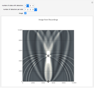 Kirchhoff Imaging
David von Seggern -
 Filtering a White-Noise Sequence
David von Seggern -
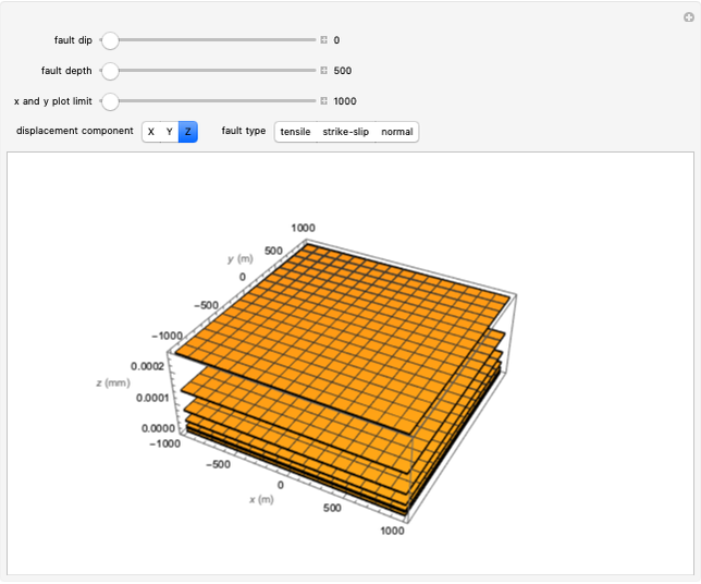 Surface Displacements Due to Underground Faults
David von Seggern -
 Shading a Surface Using Mesh
David von Seggern -
 Time Series Viewer
David von Seggern -
 Reflection and Transmission of Acoustic Waves
David von Seggern -
 Propagation of Reflected and Refracted Waves at an Interface
David von Seggern -
 Reverberations in Acoustic Layers
David von Seggern -
 Cycloid Curves
David von Seggern -
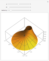 Poisson Equation on a Circular Membrane
David von Seggern -
 Laplace's Equation on a Circle
David von Seggern -
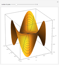
 Spherical Harmonic on Constant Latitude or Longitude
David von Seggern -
 Laplace's Equation on a Square
David von Seggern -
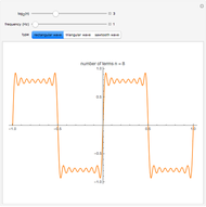 Approximation of Discontinuous Functions by Fourier Series
David von Seggern -
 Auto-Regressive Simulation (Second-Order)
David von Seggern -
Autoregressive Moving-Average Simulation (First Order)
David von Seggern