Bohm Trajectories for a Type of Derivative Nonlinear Schrödinger Equation


Requires a Wolfram Notebook System
Interact on desktop, mobile and cloud with the free Wolfram Player or other Wolfram Language products.
The time-evolution of the quantum standard wavefunction is determined by the Schrödinger equation and guidance equation. The guidance equation states that the velocity field  for the configuration is given by the quantum current
  divided by the density
  . The guidance equation is derived from the continuity equation, which is a special form of a conservation law.


Contributed by: Klaus von Bloh (March 2011)
Open content licensed under CC BY-NC-SA
Snapshots


Details
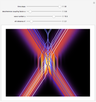
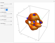
The Hirota bilinear method is applied to find exact  -soliton solutions for the DNLSE (see references). For this Demonstration a two-soliton solution is taken. The soliton has four free real parameters (
 ,
,  ,
,  ,
,  ) that characterize the velocity, the amplitude, and the width of the
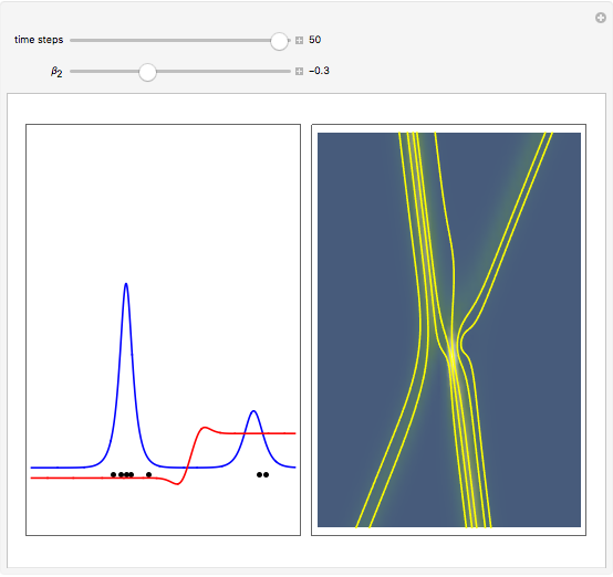
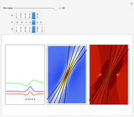
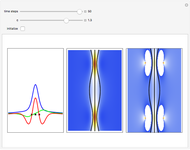
  soliton. Due to the limited CPU power, only is chosen as a free parameter. The other parameters can be found in the para options in the program. The system is time-reversible.
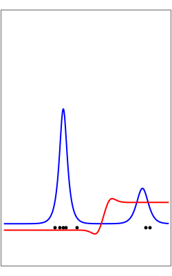
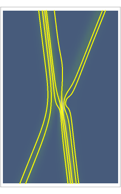
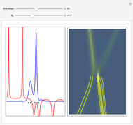
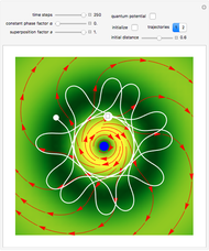
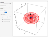
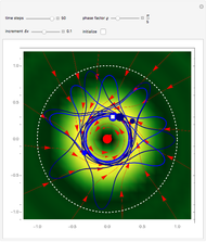
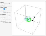
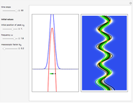
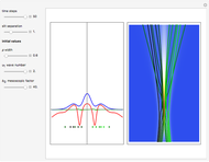
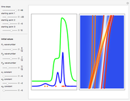
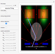
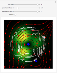
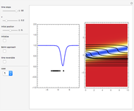
The left graphic shows the position of the particles, the wave amplitude (blue), and the velocity (red). The right graphic shows the wave amplitude and the complete trajectories in ( ,
,  ) space. The velocity is scaled to fit. In the program, if AccuracyGoal, PrecisionGoal, and MaxSteps are increased, the results will be more accurate.
References:
J. Lee, Y. Lee, and C. Lin, "Exact Solutions of DNLS and Derivative Reaction-Diffusion Systems," Journal of Nonlinear Mathematical Physics, 9(1), 2002 pp. 87–97.
W. Struyve and A. Valentini, "De Broglie-Bohm Guidance Equations for Arbitrary Hamiltonians," ArXiv:quant-ph/0808.0290v2, 2008 pp. 1–22.
Permanent Citation
 Causal Interpretation of the Nonlinear Schrödinger Equation: An Analytic Example
Klaus von Bloh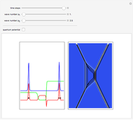 The Resonant Nonlinear Schrödinger Equation in the Causal Interpretation of Quantum Theory
Klaus von Bloh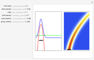 Bohm Trajectories for Quantum Particles in a Uniform Gravitational Field
Klaus von Bloh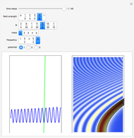 Bohm Trajectories for Quantum Airy Waves in a Time-Dependent Linear Potential
Klaus von Bloh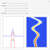 Bohm Trajectories for Quantum Particles in a Time-Dependent Linear Potential
Klaus von Bloh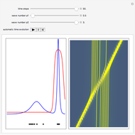 Soliton Trajectories of the Modified Korteweg-de Vries Equation (mKdV)
Klaus von Bloh Influence of the Relative Phase in the de Broglie-Bohm Theory
Klaus von Bloh Soliton Trajectories for the Kadomtsev-Petviashvili Equation
Klaus von Bloh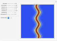 Trajectories of a Solitary Wave for the KdV Equation with Variable Coefficients
Klaus von Bloh Influence of a Moving Nodal Point on the "Causal Trajectories" in a Quantum Harmonic Oscillator Potential
Klaus von Bloh
-
 Bohm Trajectories for the Two-Dimensional Coulomb Potential
Klaus von Bloh -
 Bohm Trajectories in an LCAO Approximation for the Hydrogen Molecule H_2
Klaus von Bloh -
 Decoherence and Trajectories Implied by a Modified Schrodinger Equation
Klaus von Bloh -
 Bohm Trajectories for a Particle in a Two-Dimensional Circular Billiard
Klaus von Bloh -
 From Bohm to Classical Trajectories in a Hydrogen Atom
Klaus von Bloh -
 Continuous Transition between Quantum and Classical Behavior for a Harmonic Oscillator
Klaus von Bloh -
 Continuous Transition between Classical and Bohm Quantum Pictures for Young's Interference Experiment
Klaus von Bloh -
Bohm Trajectories for Quantum Particles in a Uniform Gravitational Field
Klaus von Bloh -
 Bohm Trajectories for a Particle in a Two-Dimensional Calogero-Moser Potential
Klaus von Bloh -
 Nonlocality in the de Broglie-Bohm Interpretation of Quantum Mechanics
Klaus von Bloh -
 Three-Soliton Collision in the Trajectory Approach
Klaus von Bloh -
 The Which-Way Experiment and the Conditional Wavefunction
Klaus von Bloh -
 Chaotic Quantum Motion of Two Particles in a 3D Harmonic Oscillator Potential
Klaus von Bloh -
 Perturbation Theory in the de Broglie-Bohm Interpretation of Quantum Mechanics
Klaus von Bloh -
 Periodic Quantum Motion of Two Particles in a 3D Harmonic Oscillator Potential
Klaus von Bloh -
 Quantum Motion of Two Particles in a 3D Trigonometric Pöschl-Teller Potential
Klaus von Bloh -
 The Talbot Carpet in the Causal Interpretation of Quantum Mechanics
Klaus von Bloh -
 Bohmian Quantum Trajectories for Coherent States of the Pöschl-Teller Potential
Klaus von Bloh -
 Gray and Dark Solitons in the de Broglie and Bohm Approaches
Klaus von Bloh -
 A Breather Solution in the Causal Interpretation of Quantum Mechanics
Klaus von Bloh